Note
Go to the end to download the full example code.
Asinh scale#
Illustration of the asinh axis scaling,
which uses the transformation
For coordinate values close to zero (i.e. much smaller than the "linear width" \(a_0\)), this leaves values essentially unchanged:
but for larger values (i.e. \(|a| \gg a_0\), this is asymptotically
As with the symlog scaling,
this allows one to plot quantities
that cover a very wide dynamic range that includes both positive
and negative values. However, symlog involves a transformation
that has discontinuities in its gradient because it is built
from separate linear and logarithmic transformations.
The asinh scaling uses a transformation that is smooth
for all (finite) values, which is both mathematically cleaner
and reduces visual artifacts associated with an abrupt
transition between linear and logarithmic regions of the plot.
Note
scale.AsinhScale is experimental, and the API may change.
See AsinhScale, SymmetricalLogScale.
import matplotlib.pyplot as plt
import numpy as np

# Prepare sample values for variations on y=x graph:
x = np.linspace(-3, 6, 500)
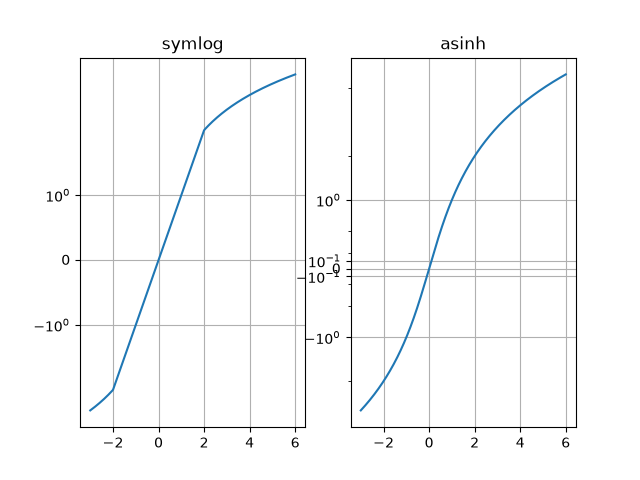
Compare "symlog" and "asinh" behaviour on sample y=x graph, where there is a discontinuous gradient in "symlog" near y=2:
fig1 = plt.figure()
ax0, ax1 = fig1.subplots(1, 2, sharex=True)

ax0.plot(x, x)
ax0.set_yscale('symlog')
ax0.grid()
ax0.set_title('symlog')

ax1.plot(x, x)
ax1.set_yscale('asinh')
ax1.grid()
ax1.set_title('asinh')
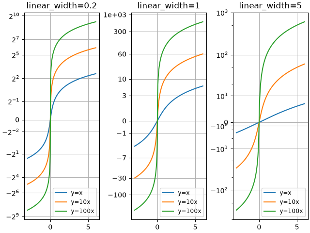
Compare "asinh" graphs with different scale parameter "linear_width":
fig2 = plt.figure(layout='constrained')
axs = fig2.subplots(1, 3, sharex=True)
for ax, (a0, base) in zip(axs, ((0.2, 2), (1.0, 0), (5.0, 10))):
    ax.set_title(f'linear_width={a0:.3g}')
    ax.plot(x, x, label='y=x')
    ax.plot(x, 10*x, label='y=10x')
    ax.plot(x, 100*x, label='y=100x')
    ax.set_yscale('asinh', linear_width=a0, base=base)
    ax.grid()
    ax.legend(loc='best', fontsize='small')
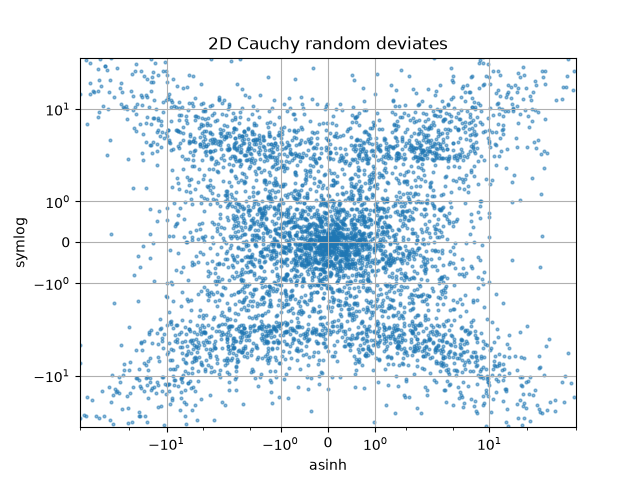
Compare "symlog" and "asinh" scalings on 2D Cauchy-distributed random numbers, where one may be able to see more subtle artifacts near y=2 due to the gradient-discontinuity in "symlog":
fig3 = plt.figure()
ax = fig3.subplots(1, 1)
r = 3 * np.tan(np.random.uniform(-np.pi / 2.02, np.pi / 2.02,
                                 size=(5000,)))
th = np.random.uniform(0, 2*np.pi, size=r.shape)

ax.scatter(r * np.cos(th), r * np.sin(th), s=4, alpha=0.5)
ax.set_xscale('asinh')
ax.set_yscale('symlog')
ax.set_xlabel('asinh')
ax.set_ylabel('symlog')
ax.set_title('2D Cauchy random deviates')
ax.set_xlim(-50, 50)
ax.set_ylim(-50, 50)
ax.grid()

plt.show()
References
Total running time of the script: (0 minutes 2.103 seconds)