Note
Go to the end to download the full example code.
Plot a confidence ellipse of a two-dimensional dataset#
This example shows how to plot a confidence ellipse of a two-dimensional dataset, using its pearson correlation coefficient.
The approach that is used to obtain the correct geometry is explained and proved here:
https://carstenschelp.github.io/2018/09/14/Plot_Confidence_Ellipse_001.html
The method avoids the use of an iterative eigen decomposition algorithm and makes use of the fact that a normalized covariance matrix (composed of pearson correlation coefficients and ones) is particularly easy to handle.
import matplotlib.pyplot as plt
import numpy as np

from matplotlib.patches import Ellipse
import matplotlib.transforms as transforms
The plotting function itself#
This function plots the confidence ellipse of the covariance of the given array-like variables x and y. The ellipse is plotted into the given Axes object ax.
The radiuses of the ellipse can be controlled by n_std which is the number of standard deviations. The default value is 3 which makes the ellipse enclose 98.9% of the points if the data is normally distributed like in these examples (3 standard deviations in 1-D contain 99.7% of the data, which is 98.9% of the data in 2-D).
def confidence_ellipse(x, y, ax, n_std=3.0, facecolor='none', **kwargs):
    """
    Create a plot of the covariance confidence ellipse of *x* and *y*.

    Parameters
    ----------
    x, y : array-like, shape (n, )
        Input data.

    ax : matplotlib.axes.Axes
        The Axes object to draw the ellipse into.

    n_std : float
        The number of standard deviations to determine the ellipse's radiuses.

    **kwargs
        Forwarded to `~matplotlib.patches.Ellipse`

    Returns
    -------
    matplotlib.patches.Ellipse
    """
    if x.size != y.size:
        raise ValueError("x and y must be the same size")

    cov = np.cov(x, y)
    pearson = cov[0, 1]/np.sqrt(cov[0, 0] * cov[1, 1])
    # Using a special case to obtain the eigenvalues of this
    # two-dimensional dataset.
    ell_radius_x = np.sqrt(1 + pearson)
    ell_radius_y = np.sqrt(1 - pearson)
    ellipse = Ellipse((0, 0), width=ell_radius_x * 2, height=ell_radius_y * 2,
                      facecolor=facecolor, **kwargs)

    # Calculating the standard deviation of x from
    # the squareroot of the variance and multiplying
    # with the given number of standard deviations.
    scale_x = np.sqrt(cov[0, 0]) * n_std
    mean_x = np.mean(x)

    # calculating the standard deviation of y ...
    scale_y = np.sqrt(cov[1, 1]) * n_std
    mean_y = np.mean(y)

    transf = transforms.Affine2D() \
        .rotate_deg(45) \
        .scale(scale_x, scale_y) \
        .translate(mean_x, mean_y)

    ellipse.set_transform(transf + ax.transData)
    return ax.add_patch(ellipse)
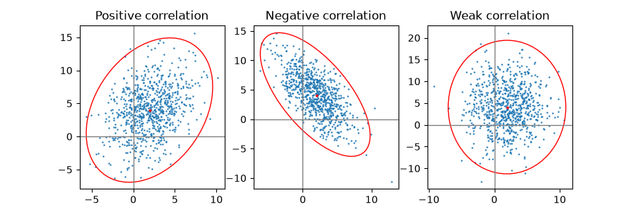
Positive, negative and weak correlation#
Note that the shape for the weak correlation (right) is an ellipse, not a circle because x and y are differently scaled. However, the fact that x and y are uncorrelated is shown by the axes of the ellipse being aligned with the x- and y-axis of the coordinate system.
np.random.seed(0)

PARAMETERS = {
    'Positive correlation': [[0.85, 0.35],
                             [0.15, -0.65]],
    'Negative correlation': [[0.9, -0.4],
                             [0.1, -0.6]],
    'Weak correlation': [[1, 0],
                         [0, 1]],
}

mu = 2, 4
scale = 3, 5

fig, axs = plt.subplots(1, 3, figsize=(9, 3))
for ax, (title, dependency) in zip(axs, PARAMETERS.items()):
    x, y = get_correlated_dataset(800, dependency, mu, scale)
    ax.scatter(x, y, s=0.5)

    ax.axvline(c='grey', lw=1)
    ax.axhline(c='grey', lw=1)

    confidence_ellipse(x, y, ax, edgecolor='red')

    ax.scatter(mu[0], mu[1], c='red', s=3)
    ax.set_title(title)

plt.show()
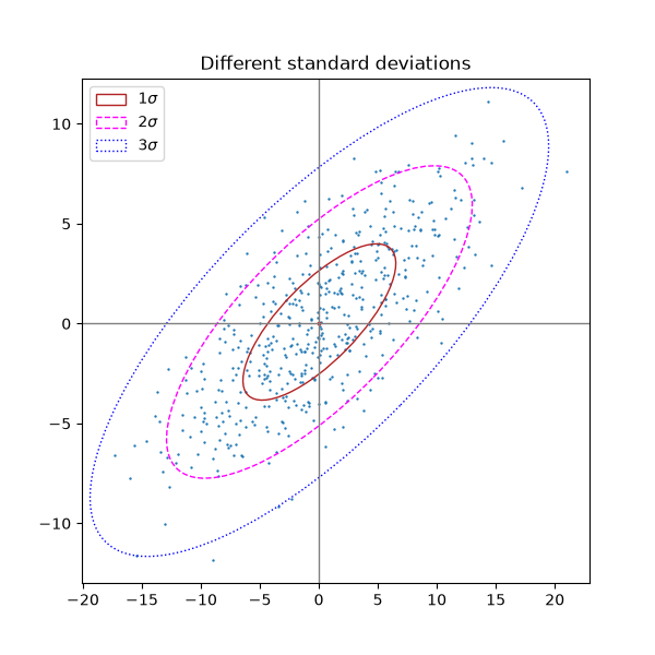
Different number of standard deviations#
A plot with n_std = 3 (blue), 2 (purple) and 1 (red)
fig, ax_nstd = plt.subplots(figsize=(6, 6))

dependency_nstd = [[0.8, 0.75],
                   [-0.2, 0.35]]
mu = 0, 0
scale = 8, 5

ax_nstd.axvline(c='grey', lw=1)
ax_nstd.axhline(c='grey', lw=1)

x, y = get_correlated_dataset(500, dependency_nstd, mu, scale)
ax_nstd.scatter(x, y, s=0.5)

confidence_ellipse(x, y, ax_nstd, n_std=1,
                   label=r'$1\sigma$', edgecolor='firebrick')
confidence_ellipse(x, y, ax_nstd, n_std=2,
                   label=r'$2\sigma$', edgecolor='fuchsia', linestyle='--')
confidence_ellipse(x, y, ax_nstd, n_std=3,
                   label=r'$3\sigma$', edgecolor='blue', linestyle=':')

ax_nstd.scatter(mu[0], mu[1], c='red', s=3)
ax_nstd.set_title('Different standard deviations')
ax_nstd.legend()
plt.show()
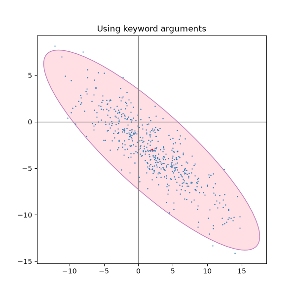
Using the keyword arguments#
Use the keyword arguments specified for matplotlib.patches.Patch in order
to have the ellipse rendered in different ways.
fig, ax_kwargs = plt.subplots(figsize=(6, 6))
dependency_kwargs = [[-0.8, 0.5],
                     [-0.2, 0.5]]
mu = 2, -3
scale = 6, 5

ax_kwargs.axvline(c='grey', lw=1)
ax_kwargs.axhline(c='grey', lw=1)

x, y = get_correlated_dataset(500, dependency_kwargs, mu, scale)
# Plot the ellipse with zorder=0 in order to demonstrate
# its transparency (caused by the use of alpha).
confidence_ellipse(x, y, ax_kwargs,
                   alpha=0.5, facecolor='pink', edgecolor='purple', zorder=0)

ax_kwargs.scatter(x, y, s=0.5)
ax_kwargs.scatter(mu[0], mu[1], c='red', s=3)
ax_kwargs.set_title('Using keyword arguments')

fig.subplots_adjust(hspace=0.25)
plt.show()
References
The use of the following functions, methods, classes and modules is shown in this example:
Total running time of the script: (0 minutes 1.568 seconds)