Note
Go to the end to download the full example code.
Contourf demo#
How to use the axes.Axes.contourf method to create filled contour plots.
import matplotlib.pyplot as plt
import numpy as np

delta = 0.025

x = y = np.arange(-3.0, 3.01, delta)
X, Y = np.meshgrid(x, y)
Z1 = np.exp(-X**2 - Y**2)
Z2 = np.exp(-(X - 1)**2 - (Y - 1)**2)
Z = (Z1 - Z2) * 2

nr, nc = Z.shape

# put NaNs in one corner:
Z[-nr // 6:, -nc // 6:] = np.nan
# contourf will convert these to masked


Z = np.ma.array(Z)
# mask another corner:
Z[:nr // 6, :nc // 6] = np.ma.masked

# mask a circle in the middle:
interior = np.sqrt(X**2 + Y**2) < 0.5
Z[interior] = np.ma.masked
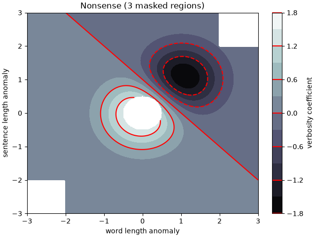
Automatic contour levels#
We are using automatic selection of contour levels; this is usually not such a good idea, because they don't occur on nice boundaries, but we do it here for purposes of illustration.
fig1, ax2 = plt.subplots(layout='constrained')
CS = ax2.contourf(X, Y, Z, 10, cmap="bone")

# Note that in the following, we explicitly pass in a subset of the contour
# levels used for the filled contours.  Alternatively, we could pass in
# additional levels to provide extra resolution, or leave out the *levels*
# keyword argument to use all of the original levels.

CS2 = ax2.contour(CS, levels=CS.levels[::2], colors='r')

ax2.set_title('Nonsense (3 masked regions)')
ax2.set_xlabel('word length anomaly')
ax2.set_ylabel('sentence length anomaly')

# Make a colorbar for the ContourSet returned by the contourf call.
cbar = fig1.colorbar(CS)
cbar.ax.set_ylabel('verbosity coefficient')
# Add the contour line levels to the colorbar
cbar.add_lines(CS2)
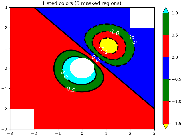
Explicit contour levels#
Now make a contour plot with the levels specified, and with the colormap generated automatically from a list of colors.
fig2, ax2 = plt.subplots(layout='constrained')
levels = [-1.5, -1, -0.5, 0, 0.5, 1]
CS3 = ax2.contourf(X, Y, Z, levels, colors=('r', 'g', 'b'), extend='both')
# Our data range extends outside the range of levels; make
# data below the lowest contour level yellow, and above the
# highest level cyan:
CS3.cmap.set_under('yellow')
CS3.cmap.set_over('cyan')

CS4 = ax2.contour(X, Y, Z, levels, colors=('k',), linewidths=(3,))
ax2.set_title('Listed colors (3 masked regions)')
ax2.clabel(CS4, fmt='%2.1f', colors='w', fontsize=14)

# Notice that the colorbar gets all the information it
# needs from the ContourSet object, CS3.
fig2.colorbar(CS3)
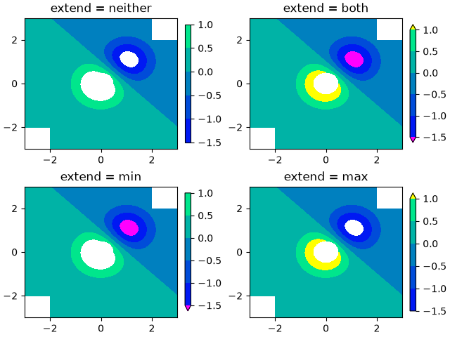
Extension settings#
Illustrate all 4 possible "extend" settings:
extends = ["neither", "both", "min", "max"]
cmap = plt.colormaps["winter"].with_extremes(under="magenta", over="yellow")
# Note: contouring simply excludes masked or nan regions, so
# instead of using the "bad" colormap value for them, it draws
# nothing at all in them.  Therefore, the following would have
# no effect:
# cmap.set_bad("red")

fig, axs = plt.subplots(2, 2, layout="constrained")

for ax, extend in zip(axs.flat, extends):
    cs = ax.contourf(X, Y, Z, levels, cmap=cmap, extend=extend)
    fig.colorbar(cs, ax=ax, shrink=0.9)
    ax.set_title("extend = %s" % extend)
    ax.locator_params(nbins=4)

plt.show()
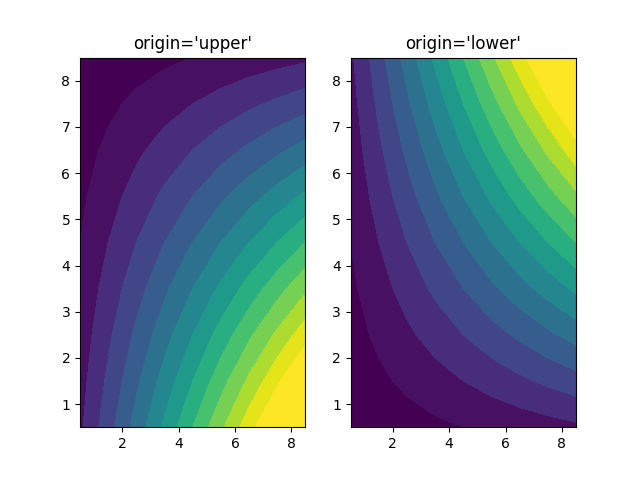
Orient contour plots using the origin keyword#
This code demonstrates orienting contour plot data using the "origin" keyword
x = np.arange(1, 10)
y = x.reshape(-1, 1)
h = x * y

fig, (ax1, ax2) = plt.subplots(ncols=2)

ax1.set_title("origin='upper'")
ax2.set_title("origin='lower'")
ax1.contourf(h, levels=np.arange(5, 70, 5), extend='both', origin="upper")
ax2.contourf(h, levels=np.arange(5, 70, 5), extend='both', origin="lower")

plt.show()
References
The use of the following functions, methods, classes and modules is shown in this example:
Total running time of the script: (0 minutes 3.422 seconds)