Note
Go to the end to download the full example code.
TickedStroke patheffect#
Matplotlib's patheffects can be used to alter the way paths
are drawn at a low enough level that they can affect almost anything.
The patheffects guide details the use of patheffects.
The TickedStroke patheffect illustrated here
draws a path with a ticked style. The spacing, length, and angle of
ticks can be controlled.
See also the Lines with a ticked patheffect example.
See also the Contouring the solution space of optimizations example.
import matplotlib.pyplot as plt
import numpy as np
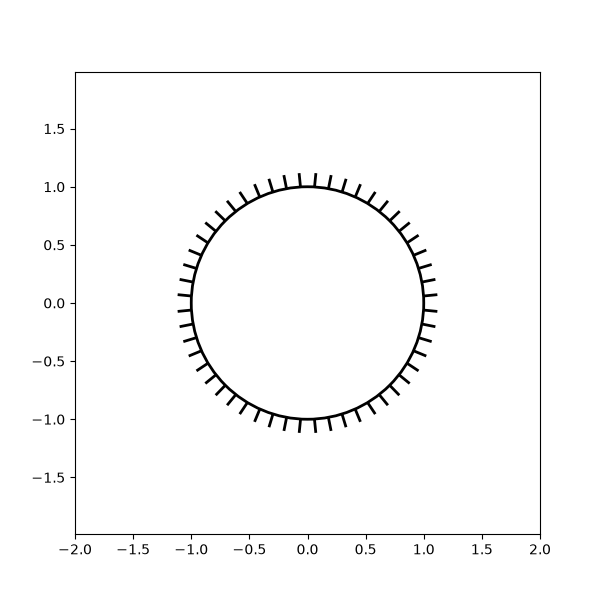
Applying TickedStroke to paths#
import matplotlib.patches as patches
from matplotlib.path import Path
import matplotlib.patheffects as patheffects

fig, ax = plt.subplots(figsize=(6, 6))
path = Path.unit_circle()
patch = patches.PathPatch(path, facecolor='none', lw=2, path_effects=[
    patheffects.withTickedStroke(angle=-90, spacing=10, length=1)])

ax.add_patch(patch)
ax.axis('equal')
ax.set_xlim(-2, 2)
ax.set_ylim(-2, 2)

plt.show()
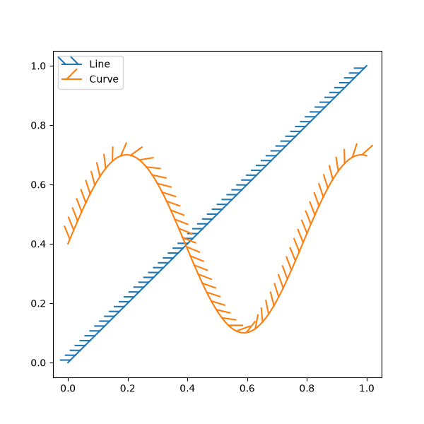
Applying TickedStroke to lines#
fig, ax = plt.subplots(figsize=(6, 6))
ax.plot([0, 1], [0, 1], label="Line",
        path_effects=[patheffects.withTickedStroke(spacing=7, angle=135)])

nx = 101
x = np.linspace(0.0, 1.0, nx)
y = 0.3*np.sin(x*8) + 0.4
ax.plot(x, y, label="Curve", path_effects=[patheffects.withTickedStroke()])

ax.legend()

plt.show()
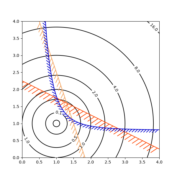
Applying TickedStroke to contour plots#
Contour plot with objective and constraints. Curves generated by contour to represent a typical constraint in an optimization problem should be plotted with angles between zero and 180 degrees.
fig, ax = plt.subplots(figsize=(6, 6))

nx = 101
ny = 105

# Set up survey vectors
xvec = np.linspace(0.001, 4.0, nx)
yvec = np.linspace(0.001, 4.0, ny)

# Set up survey matrices.  Design disk loading and gear ratio.
x1, x2 = np.meshgrid(xvec, yvec)

# Evaluate some stuff to plot
obj = x1**2 + x2**2 - 2*x1 - 2*x2 + 2
g1 = -(3*x1 + x2 - 5.5)
g2 = -(x1 + 2*x2 - 4.5)
g3 = 0.8 + x1**-3 - x2

cntr = ax.contour(x1, x2, obj, [0.01, 0.1, 0.5, 1, 2, 4, 8, 16],
                  colors='black')
ax.clabel(cntr, fmt="%2.1f", use_clabeltext=True)

cg1 = ax.contour(x1, x2, g1, [0], colors='sandybrown')
cg1.set(path_effects=[patheffects.withTickedStroke(angle=135)])

cg2 = ax.contour(x1, x2, g2, [0], colors='orangered')
cg2.set(path_effects=[patheffects.withTickedStroke(angle=60, length=2)])

cg3 = ax.contour(x1, x2, g3, [0], colors='mediumblue')
cg3.set(path_effects=[patheffects.withTickedStroke(spacing=7)])

ax.set_xlim(0, 4)
ax.set_ylim(0, 4)

plt.show()
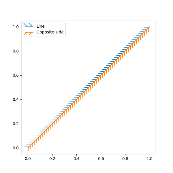
Direction/side of the ticks#
To change which side of the line the ticks are drawn, change the sign of the angle.
fig, ax = plt.subplots(figsize=(6, 6))
line_x = line_y = [0, 1]
ax.plot(line_x, line_y, label="Line",
        path_effects=[patheffects.withTickedStroke(spacing=7, angle=135)])

ax.plot(line_x, line_y, label="Opposite side",
        path_effects=[patheffects.withTickedStroke(spacing=7, angle=-135)])

ax.legend()
plt.show()
Total running time of the script: (0 minutes 1.541 seconds)