Note
Go to the end to download the full example code.
Colormap normalizations SymLogNorm#
Demonstration of using norm to map colormaps onto data in non-linear ways.
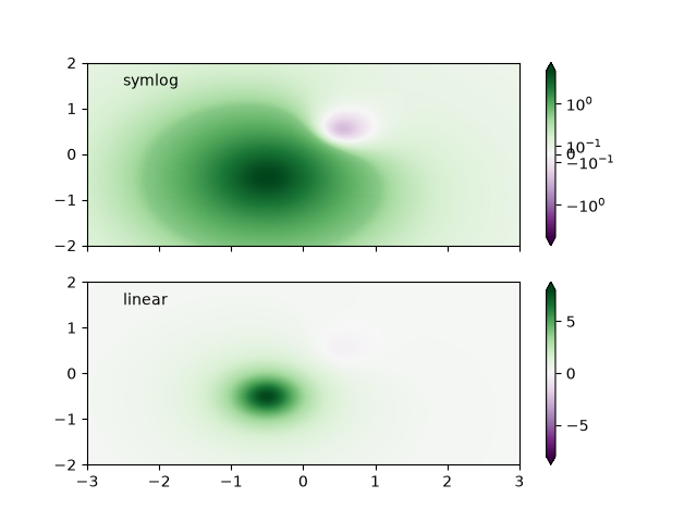
Synthetic dataset consisting of two humps, one negative and one positive, the positive with 8-times the amplitude. Linearly, the negative hump is almost invisible, and it is very difficult to see any detail of its profile. With the logarithmic scaling applied to both positive and negative values, it is much easier to see the shape of each hump.
See SymLogNorm.
import matplotlib.pyplot as plt
import numpy as np

import matplotlib.colors as colors


def rbf(x, y):
    return 1.0 / (1 + 5 * ((x ** 2) + (y ** 2)))

N = 200
gain = 8
X, Y = np.mgrid[-3:3:complex(0, N), -2:2:complex(0, N)]
Z1 = rbf(X + 0.5, Y + 0.5)
Z2 = rbf(X - 0.5, Y - 0.5)
Z = gain * Z1 - Z2

shadeopts = {'cmap': 'PRGn', 'shading': 'gouraud'}
colormap = 'PRGn'
lnrwidth = 0.5

fig, ax = plt.subplots(2, 1, sharex=True, sharey=True)

pcm = ax[0].pcolormesh(X, Y, Z,
                       norm=colors.SymLogNorm(linthresh=lnrwidth, linscale=1,
                                              vmin=-gain, vmax=gain, base=10),
                       **shadeopts)
fig.colorbar(pcm, ax=ax[0], extend='both')
ax[0].text(-2.5, 1.5, 'symlog')

pcm = ax[1].pcolormesh(X, Y, Z, vmin=-gain, vmax=gain,
                       **shadeopts)
fig.colorbar(pcm, ax=ax[1], extend='both')
ax[1].text(-2.5, 1.5, 'linear')
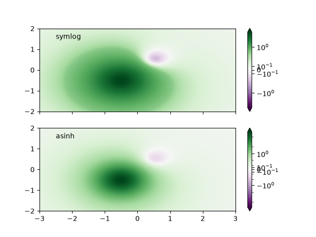
In order to find the best visualization for any particular dataset,
it may be necessary to experiment with multiple different color scales.
As well as the SymLogNorm scaling, there is also
the option of using AsinhNorm (experimental), which has a smoother
transition between the linear and logarithmic regions of the transformation
applied to the data values, "Z".
In the plots below, it may be possible to see contour-like artifacts
around each hump despite there being no sharp features
in the dataset itself. The asinh scaling shows a smoother shading
of each hump.
fig, ax = plt.subplots(2, 1, sharex=True, sharey=True)

pcm = ax[0].pcolormesh(X, Y, Z,
                       norm=colors.SymLogNorm(linthresh=lnrwidth, linscale=1,
                                              vmin=-gain, vmax=gain, base=10),
                       **shadeopts)
fig.colorbar(pcm, ax=ax[0], extend='both')
ax[0].text(-2.5, 1.5, 'symlog')

pcm = ax[1].pcolormesh(X, Y, Z,
                       norm=colors.AsinhNorm(linear_width=lnrwidth,
                                             vmin=-gain, vmax=gain),
                       **shadeopts)
fig.colorbar(pcm, ax=ax[1], extend='both')
ax[1].text(-2.5, 1.5, 'asinh')


plt.show()
Total running time of the script: (0 minutes 2.980 seconds)