Note
Go to the end to download the full example code.
Step Demo#
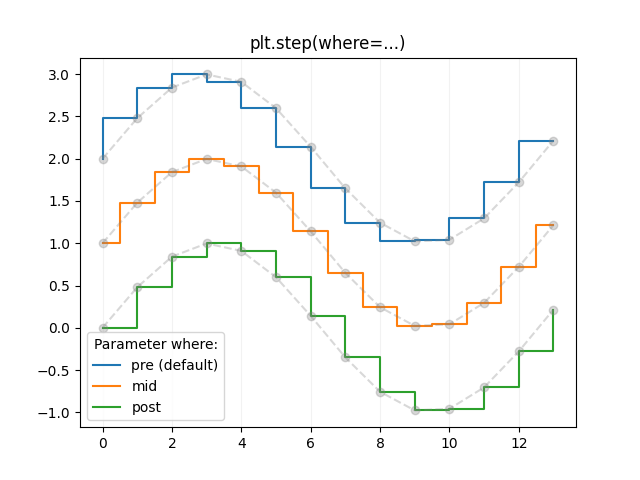
This example demonstrates the use of pyplot.step for piece-wise constant
curves. In particular, it illustrates the effect of the parameter where
on the step position.
Note
For the common case that you know the edge positions, use pyplot.stairs
instead.
The circular markers created with pyplot.plot show the actual data
positions so that it's easier to see the effect of where.
import matplotlib.pyplot as plt
import numpy as np

x = np.arange(14)
y = np.sin(x / 2)

plt.step(x, y + 2, label='pre (default)')
plt.plot(x, y + 2, 'o--', color='grey', alpha=0.3)

plt.step(x, y + 1, where='mid', label='mid')
plt.plot(x, y + 1, 'o--', color='grey', alpha=0.3)

plt.step(x, y, where='post', label='post')
plt.plot(x, y, 'o--', color='grey', alpha=0.3)

plt.grid(axis='x', color='0.95')
plt.legend(title='Parameter where:')
plt.title('plt.step(where=...)')
plt.show()
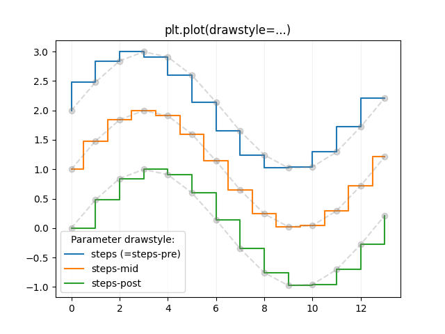
The same behavior can be achieved by using the drawstyle parameter of
pyplot.plot.
plt.plot(x, y + 2, drawstyle='steps', label='steps (=steps-pre)')
plt.plot(x, y + 2, 'o--', color='grey', alpha=0.3)

plt.plot(x, y + 1, drawstyle='steps-mid', label='steps-mid')
plt.plot(x, y + 1, 'o--', color='grey', alpha=0.3)

plt.plot(x, y, drawstyle='steps-post', label='steps-post')
plt.plot(x, y, 'o--', color='grey', alpha=0.3)

plt.grid(axis='x', color='0.95')
plt.legend(title='Parameter drawstyle:')
plt.title('plt.plot(drawstyle=...)')
plt.show()
References
The use of the following functions, methods, classes and modules is shown in this example: