Note
Click here to download the full example code
Rendering math equations using TeX
You can use TeX to render all of your Matplotlib text by setting
rcParams["text.usetex"] (default: False) to True. This requires that you have TeX and the other
dependencies described in the Text rendering with LaTeX tutorial properly
installed on your system. Matplotlib caches processed TeX expressions, so that
only the first occurrence of an expression triggers a TeX compilation. Later
occurrences reuse the rendered image from the cache and are thus faster.
Unicode input is supported, e.g. for the y-axis label in this example.
import numpy as np
import matplotlib.pyplot as plt
plt.rcParams['text.usetex'] = True
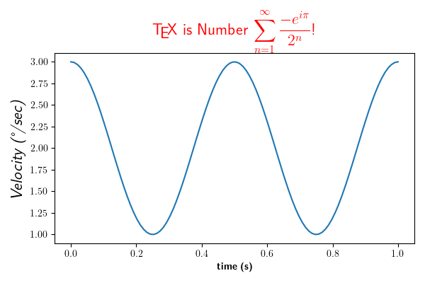
t = np.linspace(0.0, 1.0, 100)
s = np.cos(4 * np.pi * t) + 2
fig, ax = plt.subplots(figsize=(6, 4), tight_layout=True)
ax.plot(t, s)
ax.set_xlabel(r'\textbf{time (s)}')
ax.set_ylabel('\\textit{Velocity (\N{DEGREE SIGN}/sec)}', fontsize=16)
ax.set_title(r'\TeX\ is Number $\displaystyle\sum_{n=1}^\infty'
r'\frac{-e^{i\pi}}{2^n}$!', fontsize=16, color='r')
Out:
Text(0.5, 1.0652809399537557, '\\TeX\\ is Number $\\displaystyle\\sum_{n=1}^\\infty\\frac{-e^{i\\pi}}{2^n}$!')
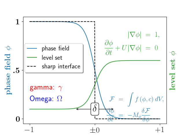
A more complex example.
fig, ax = plt.subplots()
# interface tracking profiles
N = 500
delta = 0.6
X = np.linspace(-1, 1, N)
ax.plot(X, (1 - np.tanh(4 * X / delta)) / 2,    # phase field tanh profiles
        X, (1.4 + np.tanh(4 * X / delta)) / 4, "C2",  # composition profile
        X, X < 0, "k--")                        # sharp interface

# legend
ax.legend(("phase field", "level set", "sharp interface"),
          shadow=True, loc=(0.01, 0.48), handlelength=1.5, fontsize=16)

# the arrow
ax.annotate("", xy=(-delta / 2., 0.1), xytext=(delta / 2., 0.1),
            arrowprops=dict(arrowstyle="<->", connectionstyle="arc3"))
ax.text(0, 0.1, r"$\delta$",
        color="black", fontsize=24,
        horizontalalignment="center", verticalalignment="center",
        bbox=dict(boxstyle="round", fc="white", ec="black", pad=0.2))

# Use tex in labels
ax.set_xticks([-1, 0, 1])
ax.set_xticklabels(["$-1$", r"$\pm 0$", "$+1$"], color="k", size=20)

# Left Y-axis labels, combine math mode and text mode
ax.set_ylabel(r"\bf{phase field} $\phi$", color="C0", fontsize=20)
ax.set_yticks([0, 0.5, 1])
ax.set_yticklabels([r"\bf{0}", r"\bf{.5}", r"\bf{1}"], color="k", size=20)

# Right Y-axis labels
ax.text(1.02, 0.5, r"\bf{level set} $\phi$",
        color="C2", fontsize=20, rotation=90,
        horizontalalignment="left", verticalalignment="center",
        clip_on=False, transform=ax.transAxes)

# Use multiline environment inside a `text`.
# level set equations
eq1 = (r"\begin{eqnarray*}"
       r"|\nabla\phi| &=& 1,\\"
       r"\frac{\partial \phi}{\partial t} + U|\nabla \phi| &=& 0 "
       r"\end{eqnarray*}")
ax.text(1, 0.9, eq1, color="C2", fontsize=18,
        horizontalalignment="right", verticalalignment="top")

# phase field equations
eq2 = (r"\begin{eqnarray*}"
       r"\mathcal{F} &=& \int f\left( \phi, c \right) dV, \\ "
       r"\frac{ \partial \phi } { \partial t } &=& -M_{ \phi } "
       r"\frac{ \delta \mathcal{F} } { \delta \phi }"
       r"\end{eqnarray*}")
ax.text(0.18, 0.18, eq2, color="C0", fontsize=16)

ax.text(-1, .30, r"gamma: $\gamma$", color="r", fontsize=20)
ax.text(-1, .18, r"Omega: $\Omega$", color="b", fontsize=20)

plt.show()
Total running time of the script: ( 0 minutes 1.854 seconds)
Keywords: matplotlib code example, codex, python plot, pyplot Gallery generated by Sphinx-Gallery