Note
Click here to download the full example code
The Sankey class
Demonstrate the Sankey class by producing three basic diagrams.
import matplotlib.pyplot as plt

from matplotlib.sankey import Sankey
Example 1 -- Mostly defaults
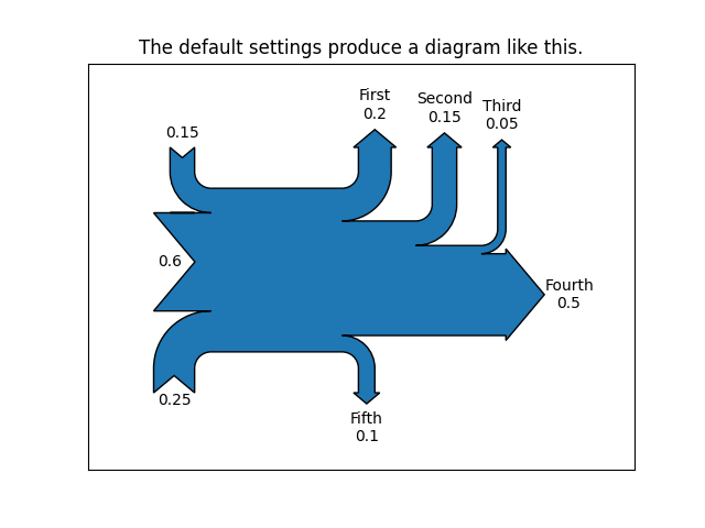
This demonstrates how to create a simple diagram by implicitly calling the Sankey.add() method and by appending finish() to the call to the class.
Out:
Text(0.5, 1.0, 'The default settings produce a diagram like this.')
Notice:
Axes weren't provided when Sankey() was instantiated, so they were created automatically.
The scale argument wasn't necessary since the data was already normalized.
By default, the lengths of the paths are justified.
Example 2
This demonstrates:
Setting one path longer than the others
Placing a label in the middle of the diagram
Using the scale argument to normalize the flows
Implicitly passing keyword arguments to PathPatch()
Changing the angle of the arrow heads
Changing the offset between the tips of the paths and their labels
Formatting the numbers in the path labels and the associated unit
Changing the appearance of the patch and the labels after the figure is created
fig = plt.figure()
ax = fig.add_subplot(1, 1, 1, xticks=[], yticks=[],
                     title="Flow Diagram of a Widget")
sankey = Sankey(ax=ax, scale=0.01, offset=0.2, head_angle=180,
                format='%.0f', unit='%')
sankey.add(flows=[25, 0, 60, -10, -20, -5, -15, -10, -40],
           labels=['', '', '', 'First', 'Second', 'Third', 'Fourth',
                   'Fifth', 'Hurray!'],
           orientations=[-1, 1, 0, 1, 1, 1, -1, -1, 0],
           pathlengths=[0.25, 0.25, 0.25, 0.25, 0.25, 0.6, 0.25, 0.25,
                        0.25],
           patchlabel="Widget\nA")  # Arguments to matplotlib.patches.PathPatch
diagrams = sankey.finish()
diagrams[0].texts[-1].set_color('r')
diagrams[0].text.set_fontweight('bold')
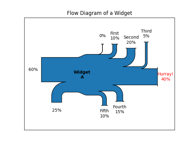
Notice:
Since the sum of the flows is nonzero, the width of the trunk isn't uniform. The matplotlib logging system logs this at the DEBUG level.
The second flow doesn't appear because its value is zero. Again, this is logged at the DEBUG level.
Example 3
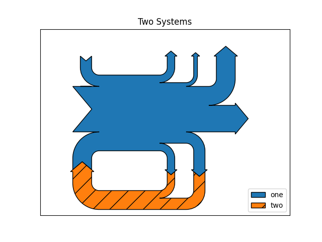
This demonstrates:
Connecting two systems
Turning off the labels of the quantities
Adding a legend
fig = plt.figure()
ax = fig.add_subplot(1, 1, 1, xticks=[], yticks=[], title="Two Systems")
flows = [0.25, 0.15, 0.60, -0.10, -0.05, -0.25, -0.15, -0.10, -0.35]
sankey = Sankey(ax=ax, unit=None)
sankey.add(flows=flows, label='one',
           orientations=[-1, 1, 0, 1, 1, 1, -1, -1, 0])
sankey.add(flows=[-0.25, 0.15, 0.1], label='two',
           orientations=[-1, -1, -1], prior=0, connect=(0, 0))
diagrams = sankey.finish()
diagrams[-1].patch.set_hatch('/')
plt.legend()
Out:
<matplotlib.legend.Legend object at 0x7fd1ee075280>
Notice that only one connection is specified, but the systems form a circuit since: (1) the lengths of the paths are justified and (2) the orientation and ordering of the flows is mirrored.
plt.show()
References
The use of the following functions, methods, classes and modules is shown in this example:
Total running time of the script: ( 0 minutes 1.337 seconds)
Keywords: matplotlib code example, codex, python plot, pyplot Gallery generated by Sphinx-Gallery