Note
Click here to download the full example code
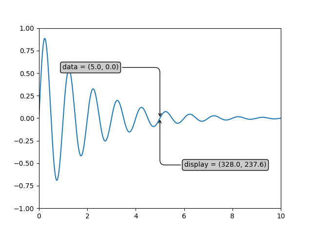
Annotate Transform#
This example shows how to use different coordinate systems for annotations. For a complete overview of the annotation capabilities, also see the annotation tutorial.
import numpy as np
import matplotlib.pyplot as plt

x = np.arange(0, 10, 0.005)
y = np.exp(-x/2.) * np.sin(2*np.pi*x)

fig, ax = plt.subplots()
ax.plot(x, y)
ax.set_xlim(0, 10)
ax.set_ylim(-1, 1)

xdata, ydata = 5, 0
xdisplay, ydisplay = ax.transData.transform((xdata, ydata))

bbox = dict(boxstyle="round", fc="0.8")
arrowprops = dict(
    arrowstyle="->",
    connectionstyle="angle,angleA=0,angleB=90,rad=10")

offset = 72
ax.annotate(
    f'data = ({xdata:.1f}, {ydata:.1f})',
    (xdata, ydata),
    xytext=(-2*offset, offset), textcoords='offset points',
    bbox=bbox, arrowprops=arrowprops)
ax.annotate(
    f'display = ({xdisplay:.1f}, {ydisplay:.1f})',
    xy=(xdisplay, ydisplay), xycoords='figure pixels',
    xytext=(0.5*offset, -offset), textcoords='offset points',
    bbox=bbox, arrowprops=arrowprops)

plt.show()
References
The use of the following functions, methods, classes and modules is shown in this example:
Keywords: matplotlib code example, codex, python plot, pyplot Gallery generated by Sphinx-Gallery