Note
Click here to download the full example code
Image antialiasing#
Images are represented by discrete pixels, either on the screen or in an image file. When data that makes up the image has a different resolution than its representation on the screen we will see aliasing effects. How noticeable these are depends on how much down-sampling takes place in the change of resolution (if any).
When subsampling data, aliasing is reduced by smoothing first and then subsampling the smoothed data. In Matplotlib, we can do that smoothing before mapping the data to colors, or we can do the smoothing on the RGB(A) data in the final image. The difference between these is shown below, and controlled with the interpolation_stage keyword argument.
The default image interpolation in Matplotlib is 'antialiased', and it is applied to the data. This uses a hanning interpolation on the data provided by the user for reduced aliasing in most situations. Only when there is upsampling by a factor of 1, 2 or >=3 is 'nearest' neighbor interpolation used.
Other anti-aliasing filters can be specified in Axes.imshow using the
interpolation keyword argument.
import numpy as np
import matplotlib.pyplot as plt
First we generate a 450x450 pixel image with varying frequency content:
N = 450
x = np.arange(N) / N - 0.5
y = np.arange(N) / N - 0.5
aa = np.ones((N, N))
aa[::2, :] = -1

X, Y = np.meshgrid(x, y)
R = np.sqrt(X**2 + Y**2)
f0 = 5
k = 100
a = np.sin(np.pi * 2 * (f0 * R + k * R**2 / 2))
# make the left hand side of this
a[:int(N / 2), :][R[:int(N / 2), :] < 0.4] = -1
a[:int(N / 2), :][R[:int(N / 2), :] < 0.3] = 1
aa[:, int(N / 3):] = a[:, int(N / 3):]
a = aa
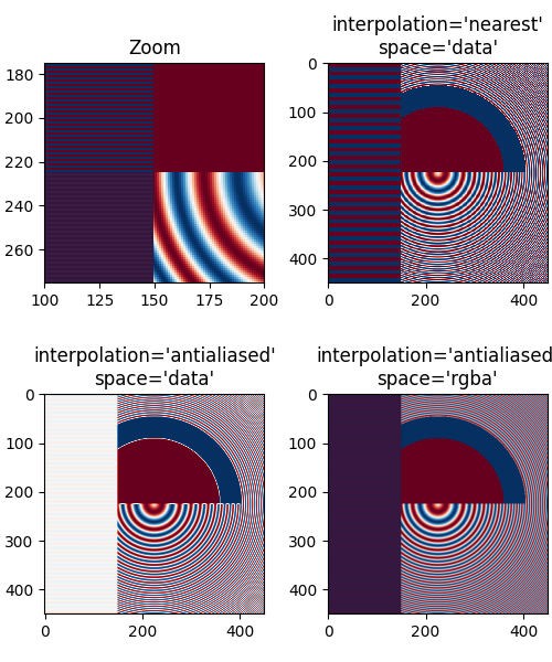
The following images are subsampled from 450 data pixels to either 125 pixels or 250 pixels (depending on your display). The Moire patterns in the 'nearest' interpolation are caused by the high-frequency data being subsampled. The 'antialiased' imaged still has some Moire patterns as well, but they are greatly reduced.
There are substantial differences between the 'data' interpolation and the 'rgba' interpolation. The alternating bands of red and blue on the left third of the image are subsampled. By interpolating in 'data' space (the default) the antialiasing filter makes the stripes close to white, because the average of -1 and +1 is zero, and zero is white in this colormap.
Conversely, when the anti-aliasing occurs in 'rgba' space, the red and blue are combined visually to make purple. This behaviour is more like a typical image processing package, but note that purple is not in the original colormap, so it is no longer possible to invert individual pixels back to their data value.
fig, axs = plt.subplots(2, 2, figsize=(5, 6), constrained_layout=True)
axs[0, 0].imshow(a, interpolation='nearest', cmap='RdBu_r')
axs[0, 0].set_xlim(100, 200)
axs[0, 0].set_ylim(275, 175)
axs[0, 0].set_title('Zoom')

for ax, interp, space in zip(axs.flat[1:],
                             ['nearest', 'antialiased', 'antialiased'],
                             ['data', 'data', 'rgba']):
    ax.imshow(a, interpolation=interp, interpolation_stage=space,
              cmap='RdBu_r')
    ax.set_title(f"interpolation='{interp}'\nspace='{space}'")
plt.show()
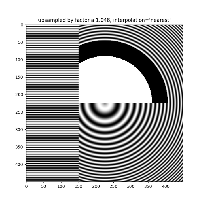
Even up-sampling an image with 'nearest' interpolation will lead to Moire patterns when the upsampling factor is not integer. The following image upsamples 500 data pixels to 530 rendered pixels. You may note a grid of 30 line-like artifacts which stem from the 524 - 500 = 24 extra pixels that had to be made up. Since interpolation is 'nearest' they are the same as a neighboring line of pixels and thus stretch the image locally so that it looks distorted.
fig, ax = plt.subplots(figsize=(6.8, 6.8))
ax.imshow(a, interpolation='nearest', cmap='gray')
ax.set_title("upsampled by factor a 1.048, interpolation='nearest'")
plt.show()
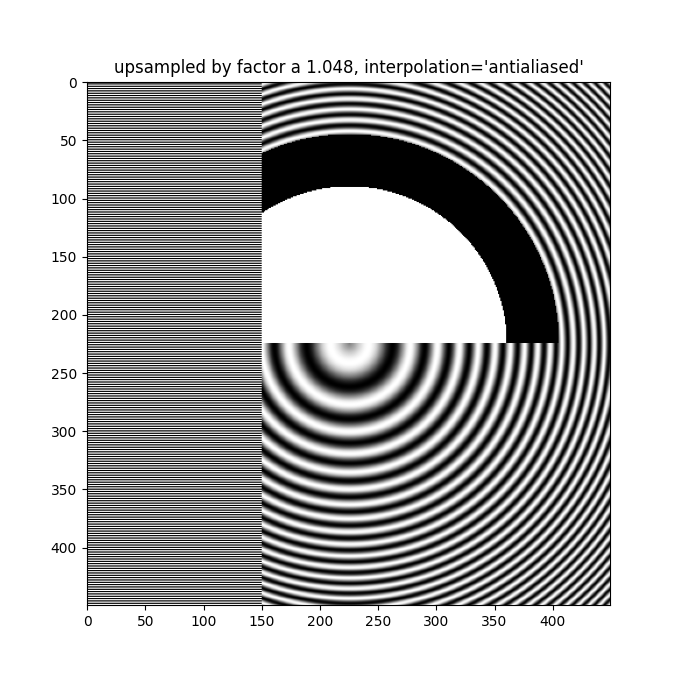
Better antialiasing algorithms can reduce this effect:
fig, ax = plt.subplots(figsize=(6.8, 6.8))
ax.imshow(a, interpolation='antialiased', cmap='gray')
ax.set_title("upsampled by factor a 1.048, interpolation='antialiased'")
plt.show()
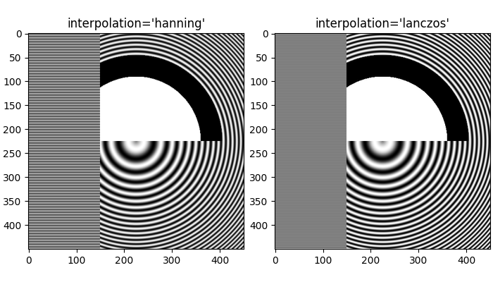
Apart from the default 'hanning' antialiasing, imshow supports a
number of different interpolation algorithms, which may work better or
worse depending on the pattern.
References
The use of the following functions, methods, classes and modules is shown in this example:
Total running time of the script: ( 0 minutes 3.108 seconds)
Keywords: matplotlib code example, codex, python plot, pyplot Gallery generated by Sphinx-Gallery