Note
Click here to download the full example code
Shading example#
Example showing how to make shaded relief plots like Mathematica or Generic Mapping Tools.
import numpy as np
from matplotlib import cbook
import matplotlib.pyplot as plt
from matplotlib.colors import LightSource
def main():
# Test data
x, y = np.mgrid[-5:5:0.05, -5:5:0.05]
z = 5 * (np.sqrt(x**2 + y**2) + np.sin(x**2 + y**2))
dem = cbook.get_sample_data('jacksboro_fault_dem.npz', np_load=True)
elev = dem['elevation']
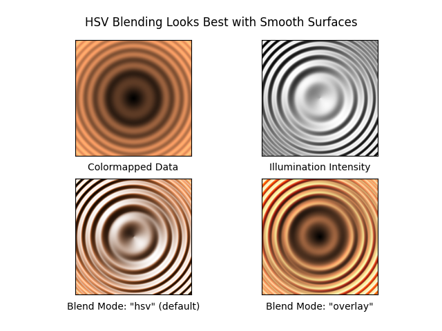
fig = compare(z, plt.cm.copper)
fig.suptitle('HSV Blending Looks Best with Smooth Surfaces', y=0.95)
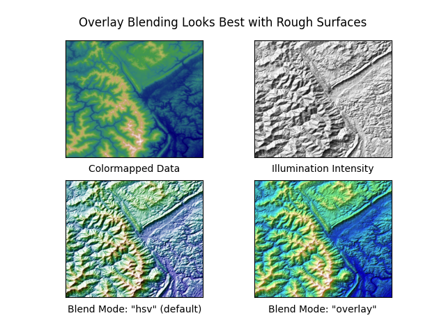
fig = compare(elev, plt.cm.gist_earth, ve=0.05)
fig.suptitle('Overlay Blending Looks Best with Rough Surfaces', y=0.95)
plt.show()
def compare(z, cmap, ve=1):
# Create subplots and hide ticks
fig, axs = plt.subplots(ncols=2, nrows=2)
for ax in axs.flat:
ax.set(xticks=[], yticks=[])
# Illuminate the scene from the northwest
ls = LightSource(azdeg=315, altdeg=45)
axs[0, 0].imshow(z, cmap=cmap)
axs[0, 0].set(xlabel='Colormapped Data')
axs[0, 1].imshow(ls.hillshade(z, vert_exag=ve), cmap='gray')
axs[0, 1].set(xlabel='Illumination Intensity')
rgb = ls.shade(z, cmap=cmap, vert_exag=ve, blend_mode='hsv')
axs[1, 0].imshow(rgb)
axs[1, 0].set(xlabel='Blend Mode: "hsv" (default)')
rgb = ls.shade(z, cmap=cmap, vert_exag=ve, blend_mode='overlay')
axs[1, 1].imshow(rgb)
axs[1, 1].set(xlabel='Blend Mode: "overlay"')
return fig
if __name__ == '__main__':
main()
References
The use of the following functions, methods, classes and modules is shown in this example:
Total running time of the script: ( 0 minutes 1.939 seconds)
Keywords: matplotlib code example, codex, python plot, pyplot Gallery generated by Sphinx-Gallery