What's new in Matplotlib 3.8.0 (Sept 13, 2023)#
For a list of all of the issues and pull requests since the last revision, see the GitHub statistics for 3.9.1 (Jul 04, 2024).
Type Hints#
Matplotlib now provides first-party PEP484 style type hints files for most public APIs.
While still considered provisional and subject to change (and sometimes we are not quite able to fully specify what we would like to), they should provide a reasonable basis to type check many common usage patterns, as well as integrating with many editors/IDEs.
Plotting and Annotation improvements#
Support customizing antialiasing for text and annotation#
matplotlib.pyplot.annotate() and matplotlib.pyplot.text() now support parameter antialiased.
When antialiased is set to True, antialiasing will be applied to the text.
When antialiased is set to False, antialiasing will not be applied to the text.
When antialiased is not specified, antialiasing will be set by rcParams["text.antialiased"] (default: True) at the creation time of Text and Annotation object.
Examples:
mpl.text.Text(.5, .5, "foo\nbar", antialiased=True)
plt.text(0.5, 0.5, '6 inches x 2 inches', antialiased=True)
ax.annotate('local max', xy=(2, 1), xytext=(3, 1.5), antialiased=False)
If the text contains math expression, antialiased applies to the whole text. Examples:
# no part will be antialiased for the text below
plt.text(0.5, 0.25, r"$I'm \sqrt{x}$", antialiased=False)
Also note that antialiasing for tick labels will be set with rcParams["text.antialiased"] (default: True) when they are created (usually when a Figure is created) and cannot be changed afterwards.
Furthermore, with this new feature, you may want to make sure that you are creating and saving/showing the figure under the same context:
# previously this was a no-op, now it is what works
with rccontext(text.antialiased=False):
    fig, ax = plt.subplots()
    ax.annotate('local max', xy=(2, 1), xytext=(3, 1.5))
    fig.savefig('/tmp/test.png')


# previously this had an effect, now this is a no-op
fig, ax = plt.subplots()
ax.annotate('local max', xy=(2, 1), xytext=(3, 1.5))
with rccontext(text.antialiased=False):
    fig.savefig('/tmp/test.png')
rcParams for AutoMinorLocator divisions#
The rcParams rcParams["xtick.minor.ndivs"] (default: 'auto') and rcParams["ytick.minor.ndivs"] (default: 'auto') have been
added to enable setting the default number of divisions; if set to auto,
the number of divisions will be chosen by the distance between major ticks.
Axline setters and getters#
The returned object from axes.Axes.axline now supports getter and setter
methods for its xy1, xy2 and slope attributes:
line1.get_xy1()
line1.get_slope()
line2.get_xy2()
line1.set_xy1(.2, .3)
line1.set_slope(2.4)
line2.set_xy2(.1, .6)
Clipping for contour plots#
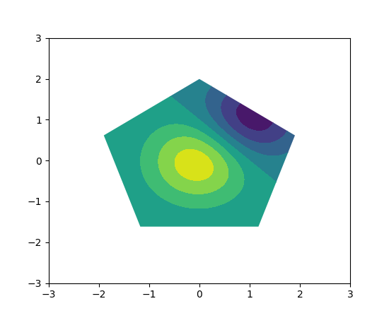
contour and contourf now accept the clip_path parameter.
import numpy as np
import matplotlib.pyplot as plt
import matplotlib.patches as mpatches

x = y = np.arange(-3.0, 3.01, 0.025)
X, Y = np.meshgrid(x, y)
Z1 = np.exp(-X**2 - Y**2)
Z2 = np.exp(-(X - 1)**2 - (Y - 1)**2)
Z = (Z1 - Z2) * 2

fig, ax = plt.subplots()
patch = mpatches.RegularPolygon((0, 0), 5, radius=2,
                                transform=ax.transData)
ax.contourf(X, Y, Z, clip_path=patch)

plt.show()
(Source code, 2x.png, png)
Axes.ecdf#
A new Axes method, ecdf, allows plotting empirical cumulative
distribution functions without any binning.
import matplotlib.pyplot as plt
import numpy as np

fig, ax = plt.subplots()
ax.ecdf(np.random.randn(100))
(Source code, 2x.png, png)
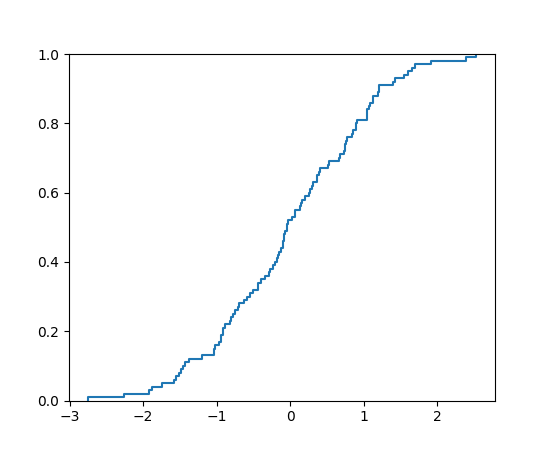
Figure.get_suptitle(), Figure.get_supxlabel(), Figure.get_supylabel()#
These methods return the strings set by Figure.suptitle(), Figure.supxlabel()
and Figure.supylabel() respectively.
Ellipse.get_vertices(), Ellipse.get_co_vertices()#
These methods return the coordinates of ellipse vertices of major and minor axis. Additionally, an example gallery demo is added which shows how to add an arrow to an ellipse showing a clockwise or counter-clockwise rotation of the ellipse. To place the arrow exactly on the ellipse, the coordinates of the vertices are used.
Remove inner ticks in label_outer()#
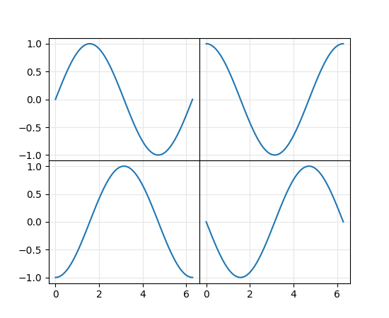
Up to now, label_outer() has only removed the ticklabels. The ticks lines
were left visible. This is now configurable through a new parameter
label_outer(remove_inner_ticks=True).
import numpy as np
import matplotlib.pyplot as plt

x = np.linspace(0, 2 * np.pi, 100)

fig, axs = plt.subplots(2, 2, sharex=True, sharey=True,
                        gridspec_kw=dict(hspace=0, wspace=0))

axs[0, 0].plot(x, np.sin(x))
axs[0, 1].plot(x, np.cos(x))
axs[1, 0].plot(x, -np.cos(x))
axs[1, 1].plot(x, -np.sin(x))

for ax in axs.flat:
    ax.grid(color='0.9')
    ax.label_outer(remove_inner_ticks=True)
(Source code, 2x.png, png)
Configurable legend shadows#
The shadow parameter of legends now accepts dicts in addition to booleans.
Dictionaries can contain any keywords for patches.Patch.
For example, this allows one to set the color and/or the transparency of a legend shadow:
ax.legend(loc='center left', shadow={'color': 'red', 'alpha': 0.5})
and to control the shadow location:
ax.legend(loc='center left', shadow={"ox":20, "oy":-20})
Configuration is currently not supported via rcParams["legend.shadow"] (default: False).
offset parameter for MultipleLocator#
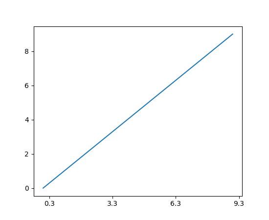
An offset may now be specified to shift all the ticks by the given value.
import matplotlib.pyplot as plt
import matplotlib.ticker as mticker

_, ax = plt.subplots()
ax.plot(range(10))
locator = mticker.MultipleLocator(base=3, offset=0.3)
ax.xaxis.set_major_locator(locator)

plt.show()
(Source code, 2x.png, png)
Add a new valid color format (matplotlib_color, alpha)#
import matplotlib.pyplot as plt
from matplotlib.patches import Rectangle

fig, ax = plt.subplots()

rectangle = Rectangle((.2, .2), .6, .6,
                      facecolor=('blue', 0.2),
                      edgecolor=('green', 0.5))
ax.add_patch(rectangle)
(Source code, 2x.png, png)
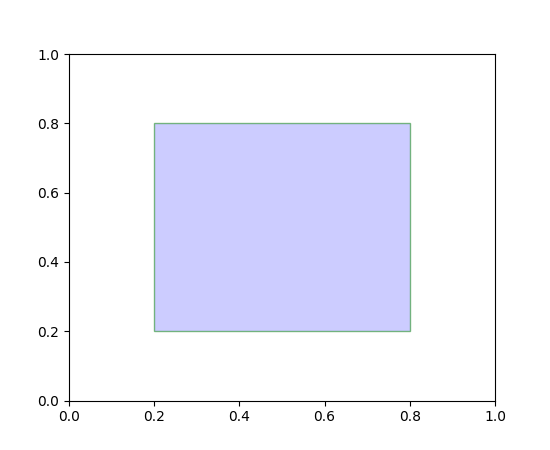
Users can define a color using the new color specification, (matplotlib_color, alpha). Note that an explicit alpha keyword argument will override an alpha value from (matplotlib_color, alpha).
The pie chart shadow can be controlled#
The shadow argument to pie can now be a dict, allowing more control
of the Shadow-patch used.
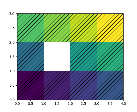
PolyQuadMesh is a new class for drawing quadrilateral meshes#
pcolor previously returned a flattened PolyCollection with only
the valid polygons (unmasked) contained within it. Now, we return a PolyQuadMesh,
which is a mixin incorporating the usefulness of 2D array and mesh coordinates
handling, but still inheriting the draw methods of PolyCollection, which enables
more control over the rendering properties than a normal QuadMesh that is
returned from pcolormesh. The new class subclasses PolyCollection and thus
should still behave the same as before. This new class keeps track of the mask for
the user and updates the Polygons that are sent to the renderer appropriately.
(Source code, 2x.png, png)
Shadow shade can be controlled#
The Shadow patch now has a shade argument to control the shadow darkness.
If 1, the shadow is black, if 0, the shadow has the same color as the patch that
is shadowed. The default value, which earlier was fixed, is 0.7.
SpinesProxy now supports calling the set() method#
One can now call e.g. ax.spines[:].set(visible=False).
Allow setting the tick label fonts with a keyword argument#
Axes.tick_params now accepts a labelfontfamily keyword that changes the tick
label font separately from the rest of the text objects:
Axis.tick_params(labelfontfamily='monospace')
Figure, Axes, and Legend Layout#
pad_inches="layout" for savefig#
When using constrained or compressed layout,
savefig(filename, bbox_inches="tight", pad_inches="layout")
will now use the padding sizes defined on the layout engine.
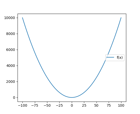
Add a public method to modify the location of Legend#
Legend locations now can be tweaked after they've been defined.
from matplotlib import pyplot as plt

fig = plt.figure()
ax = fig.add_subplot(1, 1, 1)

x = list(range(-100, 101))
y = [i**2 for i in x]

ax.plot(x, y, label="f(x)")
ax.legend()
ax.get_legend().set_loc("right")
# Or
# ax.get_legend().set(loc="right")

plt.show()
(Source code, 2x.png, png)
rcParams['legend.loc'] now accepts float-tuple inputs#
The rcParams["legend.loc"] (default: 'best') rcParams now accepts float-tuple inputs, same as the loc keyword argument to Legend.
This allows users to set the location of the legend in a more flexible and consistent way.
Mathtext improvements#
Improvements are to Mathtext, Matplotlib's native TeX-like mathematics parser (see Writing mathematical expressions, not to be confused with Matplotlib using LaTeX directly: Text rendering with LaTeX).
Boldsymbol mathtext command \boldsymbol#
Supports using the \boldsymbol{} command in mathtext:
To change symbols to bold enclose the text in a font command as shown:
r'$\boldsymbol{a+2+\alpha}$'
mathtext has more sizable delimiters#
The \lgroup and \rgroup sizable delimiters have been added.
The following delimiter names have been supported earlier, but can now be sized with
\left and \right:
\lbrace,\rbrace,\leftbrace, and\rightbrace\lbrackand\rbrack\leftparenand\rightparen
There are really no obvious advantages in using these. Instead, they are are added for completeness.
mathtext documentation improvements#
The documentation is updated to take information directly from the parser. This means that (almost) all supported symbols, operators etc are shown at Writing mathematical expressions.
mathtext now supports \substack#
\substack can be used to create multi-line subscripts or superscripts within an equation.
To use it to enclose the math in a substack command as shown:
r'$\sum_{\substack{1\leq i\leq 3\\ 1\leq j\leq 5}}$'

mathtext now supports \middle delimiter#
The \middle delimiter has been added, and can now be used with the
\left and \right delimiters:
To use the middle command enclose it in between the \left and
\right delimiter command as shown:
r'$\left( \frac{a}{b} \middle| q \right)$'

mathtext operators#
There has been a number of operators added and corrected when a Unicode font is used.
In addition, correct spacing has been added to a number of the previous operators.
Especially, the characters used for \gnapprox, \lnapprox, \leftangle, and
\rightangle have been corrected.
mathtext spacing corrections#
As consequence of the updated documentation, the spacing on a number of relational and operator symbols were classified like that and therefore will be spaced properly.
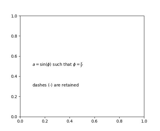
mathtext now supports \text#
\text can be used to obtain upright text within an equation and to get a plain dash
(-).
import matplotlib.pyplot as plt
plt.text(0.1, 0.5, r"$a = \sin(\phi) \text{ such that } \phi = \frac{x}{y}$")
plt.text(0.1, 0.3, r"$\text{dashes (-) are retained}$")
(Source code, 2x.png, png)
Bold-italic mathtext command \mathbfit#
Supports use of bold-italic font style in mathtext using the \mathbfit{} command:
To change font to bold and italic enclose the text in a font command as shown:
r'$\mathbfit{\eta \leq C(\delta(\eta))}$
3D plotting improvements#
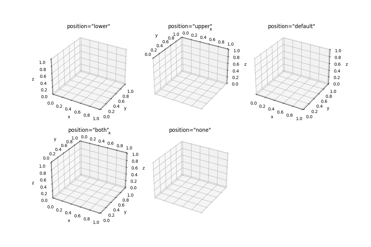
Specify ticks and axis label positions for 3D plots#
You can now specify the positions of ticks and axis labels for 3D plots.
import matplotlib.pyplot as plt

positions = ['lower', 'upper', 'default', 'both', 'none']
fig, axs = plt.subplots(2, 3, figsize=(12, 8),
                        subplot_kw={'projection': '3d'})
for ax, pos in zip(axs.flatten(), positions):
    for axis in ax.xaxis, ax.yaxis, ax.zaxis:
        axis.set_label_position(pos)
        axis.set_ticks_position(pos)
    title = f'position="{pos}"'
    ax.set(xlabel='x', ylabel='y', zlabel='z', title=title)
axs[1, 2].axis('off')
(Source code, 2x.png, png)
3D hover coordinates#
The x, y, z coordinates displayed in 3D plots were previously showing nonsensical values. This has been fixed to report the coordinate on the view pane directly beneath the mouse cursor. This is likely to be most useful when viewing 3D plots along a primary axis direction when using an orthographic projection, or when a 2D plot has been projected onto one of the 3D axis panes. Note that there is still no way to directly display the coordinates of plotted data points.
Other improvements#
macosx: New figures can be opened in either windows or tabs#
There is a new rcParams["macosx.window_mode`"] rcParam to control how
new figures are opened with the macosx backend. The default is
system which uses the system settings, or one can specify either
tab or window to explicitly choose the mode used to open new figures.
matplotlib.mpl_toolkits is now an implicit namespace package#
Following the deprecation of pkg_resources.declare_namespace in setuptools 67.3.0,
matplotlib.mpl_toolkits is now implemented as an implicit namespace, following
PEP 420.
Plot Directive now can make responsive images with "srcset"#
The plot sphinx directive (matplotlib.sphinxext.plot_directive, invoked in
rst as .. plot::) can be configured to automatically make higher res
figures and add these to the the built html docs. In conf.py:
extensions = [
...
    'matplotlib.sphinxext.plot_directive',
    'matplotlib.sphinxext.figmpl_directive',
...]

plot_srcset = ['2x']
will make png files with double the resolution for hiDPI displays. Resulting html files will have image entries like:
<img src="../_images/nestedpage-index-2.png" style="" srcset="../_images/nestedpage-index-2.png, ../_images/nestedpage-index-2.2x.png 2.00x" alt="" class="plot-directive "/>