Plotting dates and strings

The most basic way to use Matplotlib plotting methods is to pass coordinates in as numerical numpy arrays. For example, plot(x, y) will work if x and y are numpy arrays of floats (or integers). Plotting methods will also work if numpy.asarray will convert x and y to an array of floating point numbers; e.g. x could be a python list.

Matplotlib also has the ability to convert other data types if a "unit converter" exists for the data type. Matplotlib has two built-in converters, one for dates and the other for lists of strings. Other downstream libraries have their own converters to handle their data types.

The method to add converters to Matplotlib is described in matplotlib.units. Here we briefly overview the built-in date and string converters.

Date conversion

If x and/or y are a list of datetime or an array of numpy.datetime64, Matplotlib has a built-in converter that will convert the datetime to a float, and add tick locators and formatters to the axis that are appropriate for dates. See matplotlib.dates.

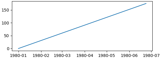
In the following example, the x-axis gains a converter that converts from numpy.datetime64 to float, and a locator that put ticks at the beginning of the month, and a formatter that label the ticks appropriately:

import numpy as np

import matplotlib.dates as mdates
import matplotlib.units as munits

import matplotlib.pyplot as plt

fig, ax = plt.subplots(figsize=(5.4, 2), layout='constrained')
time = np.arange('1980-01-01', '1980-06-25', dtype='datetime64[D]')
x = np.arange(len(time))
ax.plot(time, x)

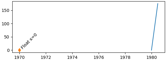
Note that if we try to plot a float on the x-axis, it will be plotted in units of days since the "epoch" for the converter, in this case 1970-01-01 (see Matplotlib date format). So when we plot the value 0, the ticks start at 1970-01-01. (The locator also now chooses every two years for a tick instead of every month):

fig, ax = plt.subplots(figsize=(5.4, 2), layout='constrained')
time = np.arange('1980-01-01', '1980-06-25', dtype='datetime64[D]')
x = np.arange(len(time))
ax.plot(time, x)
# 0 gets labeled as 1970-01-01
ax.plot(0, 0, 'd')
ax.text(0, 0, ' Float x=0', rotation=45)

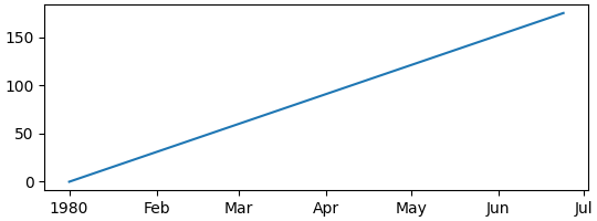
We can customize the locator and the formatter; see Date tick locators and Date formatters for a complete list, and Date tick locators and formatters for examples of them in use. Here we locate by every second month, and format just with the month's 3-letter name using "%b" (see strftime for format codes):

fig, ax = plt.subplots(figsize=(5.4, 2), layout='constrained')
time = np.arange('1980-01-01', '1980-06-25', dtype='datetime64[D]')
x = np.arange(len(time))
ax.plot(time, x)
ax.xaxis.set_major_locator(mdates.MonthLocator(bymonth=np.arange(1, 13, 2)))
ax.xaxis.set_major_formatter(mdates.DateFormatter('%b'))
ax.set_xlabel('1980')

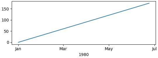
The default locator is the AutoDateLocator, and the default Formatter AutoDateFormatter. There are also "concise" formatter and locators that give a more compact labelling, and can be set via rcParams. Note how instead of the redundant "Jan" label at the start of the year, "1980" is used instead. See Formatting date ticks using ConciseDateFormatter for more examples.

plt.rcParams['date.converter'] = 'concise'

fig, ax = plt.subplots(figsize=(5.4, 2), layout='constrained')
time = np.arange('1980-01-01', '1980-06-25', dtype='datetime64[D]')
x = np.arange(len(time))
ax.plot(time, x)

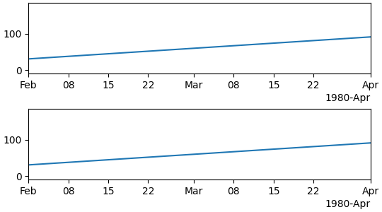
We can set the limits on the axis either by passing the appropriate dates as limits, or by passing a floating-point value in the proper units of days since the epoch. If we need it, we can get this value from date2num.

fig, axs = plt.subplots(2, 1, figsize=(5.4, 3), layout='constrained')
for ax in axs.flat:
    time = np.arange('1980-01-01', '1980-06-25', dtype='datetime64[D]')
    x = np.arange(len(time))
    ax.plot(time, x)

# set xlim using datetime64:
axs[0].set_xlim(np.datetime64('1980-02-01'), np.datetime64('1980-04-01'))

# set xlim using floats:
# Note can get from mdates.date2num(np.datetime64('1980-02-01'))
axs[1].set_xlim(3683, 3683+60)

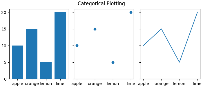
String conversion: categorical plots

Sometimes we want to label categories on an axis rather than numbers. Matplotlib allows this using a "categorical" converter (see category).

data = {'apple': 10, 'orange': 15, 'lemon': 5, 'lime': 20}
names = list(data.keys())
values = list(data.values())

fig, axs = plt.subplots(1, 3, figsize=(7, 3), sharey=True, layout='constrained')
axs[0].bar(names, values)
axs[1].scatter(names, values)
axs[2].plot(names, values)
fig.suptitle('Categorical Plotting')

Note that the "categories" are plotted in the order that they are first specified and that subsequent plotting in a different order will not affect the original order. Further, new additions will be added on the end (see "pear" below):

fig, ax = plt.subplots(figsize=(5, 3), layout='constrained')
ax.bar(names, values)

# plot in a different order:
ax.scatter(['lemon', 'apple'], [7, 12])

# add a new category, "pear", and put the other categories in a different order:
ax.plot(['pear', 'orange', 'apple', 'lemon'], [13, 10, 7, 12], color='C1')

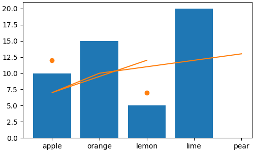
Note that when using plot like in the above, the order of the plotting is mapped onto the original order of the data, so the new line goes in the order specified.

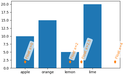
The category converter maps from categories to integers, starting at zero. So data can also be manually added to the axis using a float. Note that if a float is passed in that does not have a "category" associated with it, the data point can still be plotted, but a tick will not be created. In the following, we plot data at 4.0 and 2.5, but no tick is added there because those are not categories.

fig, ax = plt.subplots(figsize=(5, 3), layout='constrained')
ax.bar(names, values)
# arguments for styling the labels below:
args = {'rotation': 70, 'color': 'C1',
        'bbox': {'color': 'white', 'alpha': .7, 'boxstyle': 'round'}}


# 0 gets labeled as "apple"
ax.plot(0, 2, 'd', color='C1')
ax.text(0, 3, 'Float x=0', **args)

# 2 gets labeled as "lemon"
ax.plot(2, 2, 'd', color='C1')
ax.text(2, 3, 'Float x=2', **args)

# 4 doesn't get a label
ax.plot(4, 2, 'd', color='C1')
ax.text(4, 3, 'Float x=4', **args)

# 2.5 doesn't get a label
ax.plot(2.5, 2, 'd', color='C1')
ax.text(2.5, 3, 'Float x=2.5', **args)

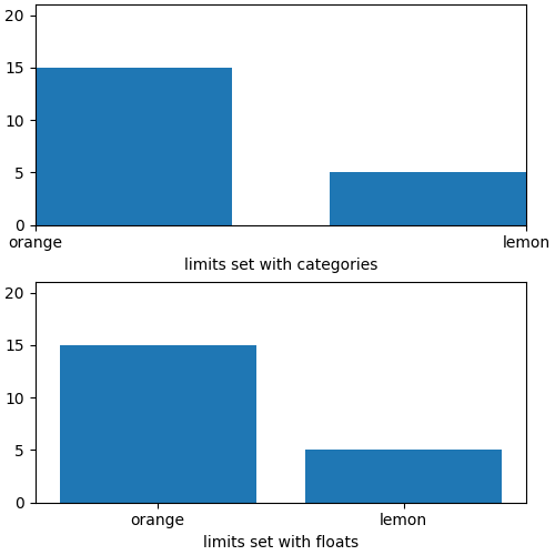
Setting the limits for a category axis can be done by specifying the categories, or by specifying floating point numbers:

fig, axs = plt.subplots(2, 1, figsize=(5, 5), layout='constrained')
ax = axs[0]
ax.bar(names, values)
ax.set_xlim('orange', 'lemon')
ax.set_xlabel('limits set with categories')
ax = axs[1]
ax.bar(names, values)
ax.set_xlim(0.5, 2.5)
ax.set_xlabel('limits set with floats')

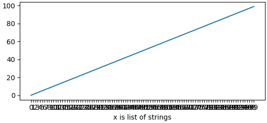
The category axes are helpful for some plot types, but can lead to confusion if data is read in as a list of strings, even if it is meant to be a list of floats or dates. This sometimes happens when reading comma-separated value (CSV) files. The categorical locator and formatter will put a tick at every string value and label each one as well:

fig, ax = plt.subplots(figsize=(5.4, 2.5), layout='constrained')
x = [str(xx) for xx in np.arange(100)]  # list of strings
ax.plot(x, np.arange(100))
ax.set_xlabel('x is list of strings')

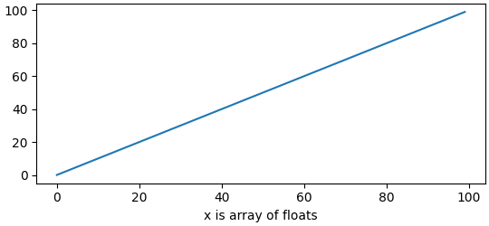
If this is not desired, then simply convert the data to floats before plotting:

fig, ax = plt.subplots(figsize=(5.4, 2.5), layout='constrained')
x = np.asarray(x, dtype='float')  # array of float.
ax.plot(x, np.arange(100))
ax.set_xlabel('x is array of floats')

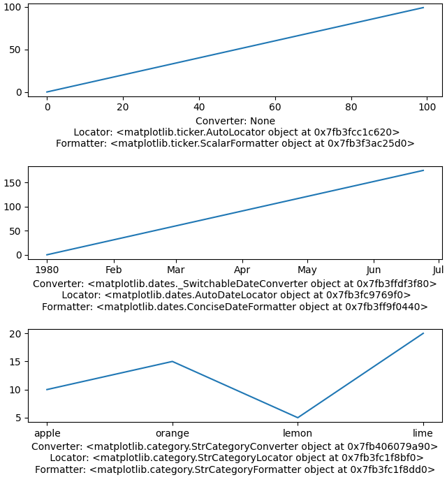
Determine converter, formatter, and locator on an axis

Sometimes it is helpful to be able to debug what Matplotlib is using to convert the incoming data. We can do that by querying the converter property on the axis. We can also query the formatters and locators using get_major_locator and get_major_formatter.

Note that by default the converter is None.

fig, axs = plt.subplots(3, 1, figsize=(6.4, 7), layout='constrained')
x = np.arange(100)
ax = axs[0]
ax.plot(x, x)
label = f'Converter: {ax.xaxis.converter}\n '
label += f'Locator: {ax.xaxis.get_major_locator()}\n'
label += f'Formatter: {ax.xaxis.get_major_formatter()}\n'
ax.set_xlabel(label)

ax = axs[1]
time = np.arange('1980-01-01', '1980-06-25', dtype='datetime64[D]')
x = np.arange(len(time))
ax.plot(time, x)
label = f'Converter: {ax.xaxis.converter}\n '
label += f'Locator: {ax.xaxis.get_major_locator()}\n'
label += f'Formatter: {ax.xaxis.get_major_formatter()}\n'
ax.set_xlabel(label)

ax = axs[2]
data = {'apple': 10, 'orange': 15, 'lemon': 5, 'lime': 20}
names = list(data.keys())
values = list(data.values())
ax.plot(names, values)
label = f'Converter: {ax.xaxis.converter}\n '
label += f'Locator: {ax.xaxis.get_major_locator()}\n'
label += f'Formatter: {ax.xaxis.get_major_formatter()}\n'
ax.set_xlabel(label)

More about "unit" support

The support for dates and categories is part of "units" support that is built into Matplotlib. This is described at matplotlib.units and in the Basic Units example.

Unit support works by querying the type of data passed to the plotting function and dispatching to the first converter in a list that accepts that type of data. So below, if x has datetime objects in it, the converter will be _SwitchableDateConverter; if it has has strings in it, it will be sent to the StrCategoryConverter.

for k, v in munits.registry.items():
    print(f"type: {k};\n    converter: {type(v)}")

type: <class 'decimal.Decimal'>;
    converter: <class 'matplotlib.units.DecimalConverter'>
type: <class 'numpy.datetime64'>;
    converter: <class 'matplotlib.dates._SwitchableDateConverter'>
type: <class 'datetime.date'>;
    converter: <class 'matplotlib.dates._SwitchableDateConverter'>
type: <class 'datetime.datetime'>;
    converter: <class 'matplotlib.dates._SwitchableDateConverter'>
type: <class 'str'>;
    converter: <class 'matplotlib.category.StrCategoryConverter'>
type: <class 'numpy.str_'>;
    converter: <class 'matplotlib.category.StrCategoryConverter'>
type: <class 'bytes'>;
    converter: <class 'matplotlib.category.StrCategoryConverter'>
type: <class 'numpy.bytes_'>;
    converter: <class 'matplotlib.category.StrCategoryConverter'>

There are a number of downstream libraries that provide their own converters with locators and formatters. Physical unit support is provided by astropy, pint, and unyt, among others.

High level libraries like pandas and nc-time-axis (and thus xarray) provide their own datetime support. This support can sometimes be incompatible with Matplotlib native datetime support, so care should be taken when using Matplotlib locators and formatters if these libraries are being used.