What's new in Matplotlib 3.6.0 (Sep 15, 2022)#
For a list of all of the issues and pull requests since the last revision, see the GitHub statistics for 3.6.0 (Sep 15, 2022).
Figure and Axes creation / management#
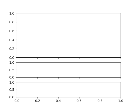
subplots, subplot_mosaic accept height_ratios and width_ratios arguments#
The relative width and height of columns and rows in subplots and
subplot_mosaic can be controlled by passing height_ratios and
width_ratios keyword arguments to the methods:
fig = plt.figure()
axs = fig.subplots(3, 1, sharex=True, height_ratios=[3, 1, 1])
(Source code, png)

Previously, this required passing the ratios in gridspec_kw arguments:
fig = plt.figure()
axs = fig.subplots(3, 1, sharex=True,
                   gridspec_kw=dict(height_ratios=[3, 1, 1]))
Constrained layout is no longer considered experimental#
The constrained layout engine and API is no longer considered experimental. Arbitrary changes to behaviour and API are no longer permitted without a deprecation period.
New layout_engine module#
Matplotlib ships with tight_layout and constrained_layout layout
engines. A new layout_engine module is provided to allow downstream
libraries to write their own layout engines and Figure objects can
now take a LayoutEngine subclass as an argument to the layout parameter.
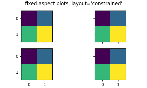
Compressed layout for fixed-aspect ratio Axes#
Simple arrangements of Axes with fixed aspect ratios can now be packed together
with fig, axs = plt.subplots(2, 3, layout='compressed').
With layout='tight' or 'constrained', Axes with a fixed aspect ratio
can leave large gaps between each other:
(Source code, png)

Using the layout='compressed' layout reduces the space between the Axes,
and adds the extra space to the outer margins:
(Source code, png)
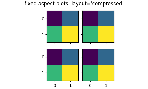
See Grids of fixed aspect-ratio Axes: "compressed" layout for further details.
Layout engines may now be removed#
The layout engine on a Figure may now be removed by calling
Figure.set_layout_engine with 'none'. This may be useful after computing
layout in order to reduce computations, e.g., for subsequent animation loops.
A different layout engine may be set afterwards, so long as it is compatible with the previous layout engine.
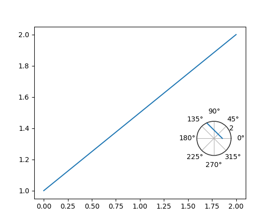
Axes.inset_axes flexibility#
matplotlib.axes.Axes.inset_axes now accepts the projection, polar and
axes_class keyword arguments, so that subclasses of matplotlib.axes.Axes
may be returned.
fig, ax = plt.subplots()

ax.plot([0, 2], [1, 2])

polar_ax = ax.inset_axes([0.75, 0.25, 0.2, 0.2], projection='polar')
polar_ax.plot([0, 2], [1, 2])
(Source code, png)
WebP is now a supported output format#
Figures may now be saved in WebP format by using the .webp file extension,
or passing format='webp' to savefig. This relies on Pillow support for WebP.
Garbage collection is no longer run on figure close#
Matplotlib has a large number of circular references (between Figure and Manager, between Axes and Figure, Axes and Artist, Figure and Canvas, etc.) so when the user drops their last reference to a Figure (and clears it from pyplot's state), the objects will not immediately be deleted.
To account for this we have long (since before 2004) had a gc.collect (of the
lowest two generations only) in the closing code in order to promptly clean up
after ourselves. However this is both not doing what we want (as most of our
objects will actually survive) and due to clearing out the first generation
opened us up to having unbounded memory usage.
In cases with a very tight loop between creating the figure and destroying it
(e.g. plt.figure(); plt.close()) the first generation will never grow large
enough for Python to consider running the collection on the higher generations.
This will lead to unbounded memory usage as the long-lived objects are never
re-considered to look for reference cycles and hence are never deleted.
We now no longer do any garbage collection when a figure is closed, and rely on
Python automatically deciding to run garbage collection periodically. If you
have strict memory requirements, you can call gc.collect yourself but this
may have performance impacts in a tight computation loop.
Plotting methods#
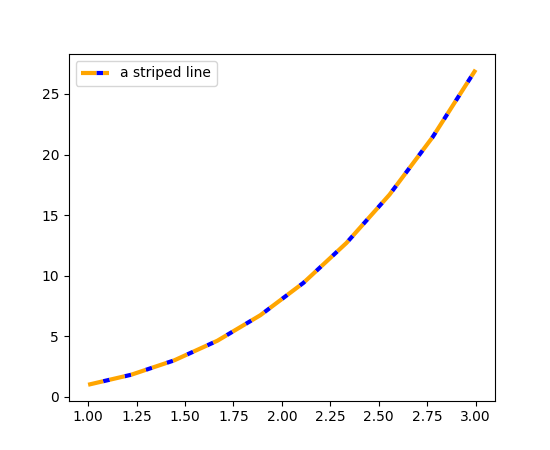
Striped lines (experimental)#
The new gapcolor parameter to plot enables the creation of striped
lines.
x = np.linspace(1., 3., 10)
y = x**3

fig, ax = plt.subplots()
ax.plot(x, y, linestyle='--', color='orange', gapcolor='blue',
        linewidth=3, label='a striped line')
ax.legend()
(Source code, png)
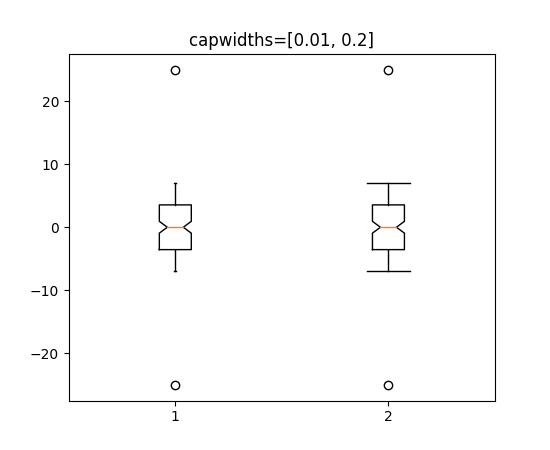
Custom cap widths in box and whisker plots in bxp and boxplot#
The new capwidths parameter to bxp and boxplot allows
controlling the widths of the caps in box and whisker plots.
x = np.linspace(-7, 7, 140)
x = np.hstack([-25, x, 25])
capwidths = [0.01, 0.2]

fig, ax = plt.subplots()
ax.boxplot([x, x], notch=True, capwidths=capwidths)
ax.set_title(f'{capwidths=}')
(Source code, png)

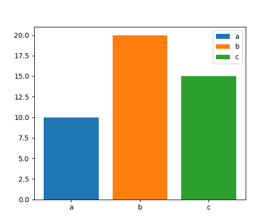
Easier labelling of bars in bar plot#
The label argument of bar and barh can now be passed a list
of labels for the bars. The list must be the same length as x and labels the
individual bars. Repeated labels are not de-duplicated and will cause repeated
label entries, so this is best used when bars also differ in style (e.g., by
passing a list to color, as below.)
x = ["a", "b", "c"]
y = [10, 20, 15]
color = ['C0', 'C1', 'C2']

fig, ax = plt.subplots()
ax.bar(x, y, color=color, label=x)
ax.legend()
(Source code, png)

New style format string for colorbar ticks#
The format argument of colorbar (and other colorbar methods) now
accepts {}-style format strings.
fig, ax = plt.subplots()
im = ax.imshow(z)
fig.colorbar(im, format='{x:.2e}')  # Instead of '%.2e'
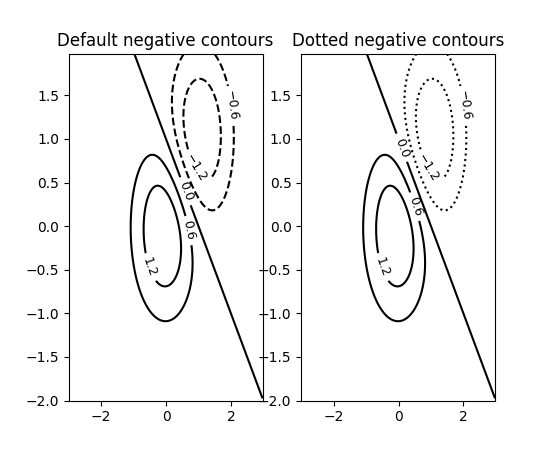
Linestyles for negative contours may be set individually#
The line style of negative contours may be set by passing the
negative_linestyles argument to Axes.contour. Previously, this style could
only be set globally via rcParams["contour.negative_linestyles"].
delta = 0.025
x = np.arange(-3.0, 3.0, delta)
y = np.arange(-2.0, 2.0, delta)
X, Y = np.meshgrid(x, y)
Z1 = np.exp(-X**2 - Y**2)
Z2 = np.exp(-(X - 1)**2 - (Y - 1)**2)
Z = (Z1 - Z2) * 2

fig, axs = plt.subplots(1, 2)

CS = axs[0].contour(X, Y, Z, 6, colors='k')
axs[0].clabel(CS, fontsize=9, inline=True)
axs[0].set_title('Default negative contours')

CS = axs[1].contour(X, Y, Z, 6, colors='k', negative_linestyles='dotted')
axs[1].clabel(CS, fontsize=9, inline=True)
axs[1].set_title('Dotted negative contours')
(Source code, png)

Improved quad contour calculations via ContourPy#
The contouring functions contour and contourf have
a new keyword argument algorithm to control which algorithm is used to
calculate the contours. There is a choice of four algorithms to use, and the
default is to use algorithm='mpl2014' which is the same algorithm that
Matplotlib has been using since 2014.
Previously Matplotlib shipped its own C++ code for calculating the contours of quad grids. Now the external library ContourPy is used instead.
Other possible values of the algorithm keyword argument at this time are
'mpl2005', 'serial' and 'threaded'; see the ContourPy
documentation for further details.
Note
Contour lines and polygons produced by algorithm='mpl2014' will be the
same as those produced before this change to within floating-point
tolerance. The exception is for duplicate points, i.e. contours containing
adjacent (x, y) points that are identical; previously the duplicate points
were removed, now they are kept. Contours affected by this will produce the
same visual output, but there will be a greater number of points in the
contours.
The locations of contour labels obtained by using clabel may
also be different.
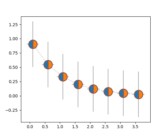
errorbar supports markerfacecoloralt#
The markerfacecoloralt parameter is now passed to the line plotter from
Axes.errorbar. The documentation now accurately lists which properties are
passed to Line2D, rather than claiming that all keyword arguments are passed
on.
x = np.arange(0.1, 4, 0.5)
y = np.exp(-x)

fig, ax = plt.subplots()
ax.errorbar(x, y, xerr=0.2, yerr=0.4,
            linestyle=':', color='darkgrey',
            marker='o', markersize=20, fillstyle='left',
            markerfacecolor='tab:blue', markerfacecoloralt='tab:orange',
            markeredgecolor='tab:brown', markeredgewidth=2)
(Source code, png)

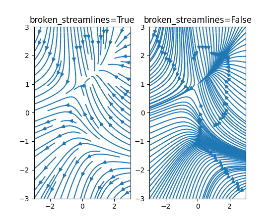
streamplot can disable streamline breaks#
It is now possible to specify that streamplots have continuous, unbroken streamlines. Previously streamlines would end to limit the number of lines within a single grid cell. See the difference between the plots below:
(Source code, png)

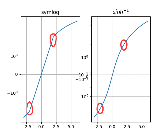
New axis scale asinh (experimental)#
The new asinh axis scale offers an alternative to symlog that smoothly
transitions between the quasi-linear and asymptotically logarithmic regions of
the scale. This is based on an arcsinh transformation that allows plotting both
positive and negative values that span many orders of magnitude.
(Source code, png)

stairs(..., fill=True) hides patch edge by setting linewidth#
stairs(..., fill=True) would previously hide Patch edges by setting
edgecolor="none". Consequently, calling set_color() on the Patch later
would make the Patch appear larger.
Now, by using linewidth=0, this apparent size change is prevented. Likewise
calling stairs(..., fill=True, linewidth=3) will behave more transparently.
Fix the dash offset of the Patch class#
Formerly, when setting the line style on a Patch object using a dash tuple,
the offset was ignored. Now the offset is applied to the Patch as expected and
it can be used as it is used with Line2D objects.
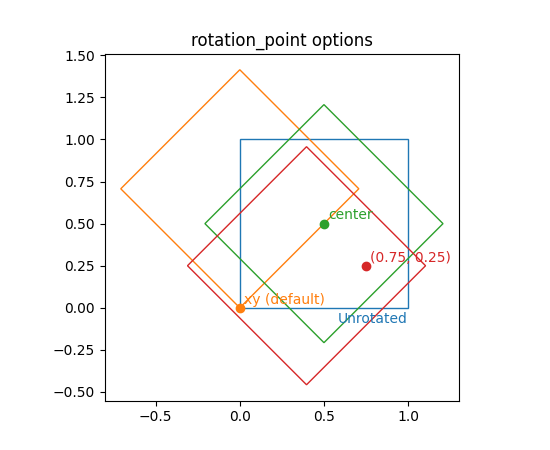
Rectangle patch rotation point#
The rotation point of the Rectangle can now be set to
'xy', 'center' or a 2-tuple of numbers using the rotation_point argument.
(Source code, png)
Colors and colormaps#
Color sequence registry#
The color sequence registry, ColorSequenceRegistry, contains sequences
(i.e., simple lists) of colors that are known to Matplotlib by name. This will
not normally be used directly, but through the universal instance at
matplotlib.color_sequences.
Colormap method for creating a different lookup table size#
The new method Colormap.resampled creates a new Colormap instance
with the specified lookup table size. This is a replacement for manipulating
the lookup table size via get_cmap.
Use:
get_cmap(name).resampled(N)
instead of:
get_cmap(name, lut=N)
Setting norms with strings#
Norms can now be set (e.g. on images) using the string name of the
corresponding scale, e.g. imshow(array, norm="log"). Note that in that
case, it is permissible to also pass vmin and vmax, as a new Norm instance
will be created under the hood.
Titles, ticks, and labels#
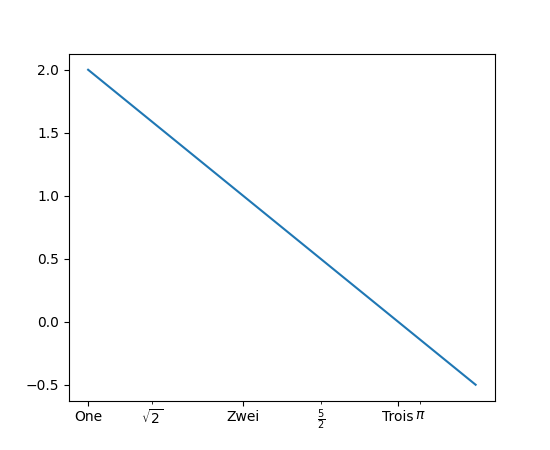
plt.xticks and plt.yticks support minor keyword argument#
It is now possible to set or get minor ticks using pyplot.xticks and
pyplot.yticks by setting minor=True.
plt.figure()
plt.plot([1, 2, 3, 3.5], [2, 1, 0, -0.5])
plt.xticks([1, 2, 3], ["One", "Zwei", "Trois"])
plt.xticks([np.sqrt(2), 2.5, np.pi],
           [r"$\sqrt{2}$", r"$\frac{5}{2}$", r"$\pi$"], minor=True)
(Source code, png)
Legends#
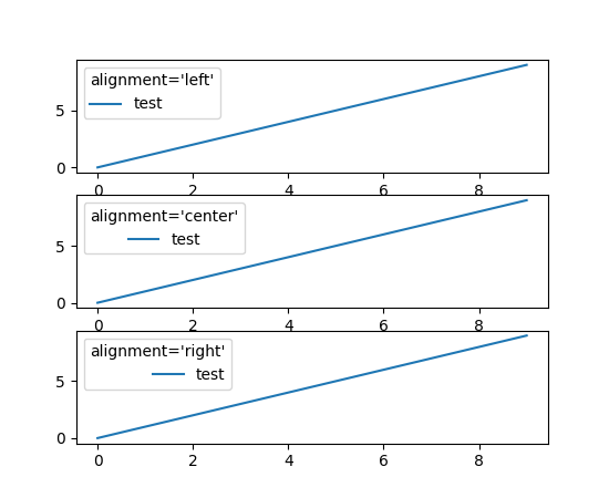
Legend can control alignment of title and handles#
Legend now supports controlling the alignment of the title and handles via
the keyword argument alignment. You can also use Legend.set_alignment to
control the alignment on existing Legends.
fig, axs = plt.subplots(3, 1)
for i, alignment in enumerate(['left', 'center', 'right']):
    axs[i].plot(range(10), label='test')
    axs[i].legend(title=f'{alignment=}', alignment=alignment)
(Source code, png)
ncol keyword argument to legend renamed to ncols#
The ncol keyword argument to legend for controlling the number of
columns is renamed to ncols for consistency with the ncols and nrows
keywords of subplots and GridSpec. ncol remains supported for
backwards compatibility, but is discouraged.
Markers#
marker can now be set to the string "none"#
The string "none" means no-marker, consistent with other APIs which support the lowercase version. Using "none" is recommended over using "None", to avoid confusion with the None object.
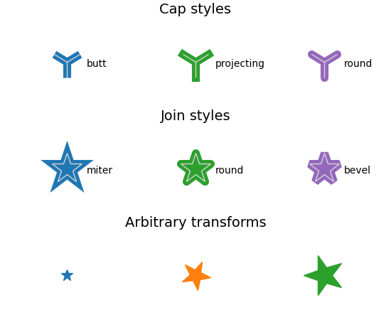
Customization of MarkerStyle join and cap style#
New MarkerStyle parameters allow control of join style and cap style, and
for the user to supply a transformation to be applied to the marker (e.g. a
rotation).
from matplotlib.markers import CapStyle, JoinStyle, MarkerStyle
from matplotlib.transforms import Affine2D

fig, axs = plt.subplots(3, 1, layout='constrained')
for ax in axs:
    ax.axis('off')
    ax.set_xlim(-0.5, 2.5)

axs[0].set_title('Cap styles', fontsize=14)
for col, cap in enumerate(CapStyle):
    axs[0].plot(col, 0, markersize=32, markeredgewidth=8,
                marker=MarkerStyle('1', capstyle=cap))
    # Show the marker edge for comparison with the cap.
    axs[0].plot(col, 0, markersize=32, markeredgewidth=1,
                markerfacecolor='none', markeredgecolor='lightgrey',
                marker=MarkerStyle('1'))
    axs[0].annotate(cap.name, (col, 0),
                    xytext=(20, -5), textcoords='offset points')

axs[1].set_title('Join styles', fontsize=14)
for col, join in enumerate(JoinStyle):
    axs[1].plot(col, 0, markersize=32, markeredgewidth=8,
                marker=MarkerStyle('*', joinstyle=join))
    # Show the marker edge for comparison with the join.
    axs[1].plot(col, 0, markersize=32, markeredgewidth=1,
                markerfacecolor='none', markeredgecolor='lightgrey',
                marker=MarkerStyle('*'))
    axs[1].annotate(join.name, (col, 0),
                    xytext=(20, -5), textcoords='offset points')

axs[2].set_title('Arbitrary transforms', fontsize=14)
for col, (size, rot) in enumerate(zip([2, 5, 7], [0, 45, 90])):
    t = Affine2D().rotate_deg(rot).scale(size)
    axs[2].plot(col, 0, marker=MarkerStyle('*', transform=t))
(Source code, png)

Fonts and Text#
Font fallback#
It is now possible to specify a list of fonts families and Matplotlib will try them in order to locate a required glyph.
plt.rcParams["font.size"] = 20
fig = plt.figure(figsize=(4.75, 1.85))

text = "There are 几个汉字 in between!"
fig.text(0.05, 0.85, text, family=["WenQuanYi Zen Hei"])
fig.text(0.05, 0.65, text, family=["Noto Sans CJK JP"])
fig.text(0.05, 0.45, text, family=["DejaVu Sans", "Noto Sans CJK JP"])
fig.text(0.05, 0.25, text, family=["DejaVu Sans", "WenQuanYi Zen Hei"])
(Source code, png)
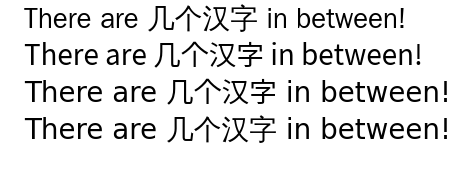
Demonstration of mixed English and Chinese text with font fallback.#
This currently works with the Agg (and all of the GUI embeddings), svg, pdf, ps, and inline backends.
List of available font names#
The list of available fonts are now easily accessible. To get a list of the available font names in Matplotlib use:
from matplotlib import font_manager
font_manager.get_font_names()
math_to_image now has a color keyword argument#
To easily support external libraries that rely on the MathText rendering of
Matplotlib to generate equation images, a color keyword argument was added to
math_to_image.
from matplotlib import mathtext
mathtext.math_to_image('$x^2$', 'filename.png', color='Maroon')
Active URL area rotates with link text#
When link text is rotated in a figure, the active URL area will now include the rotated link area. Previously, the active area remained in the original, non-rotated, position.
rcParams improvements#
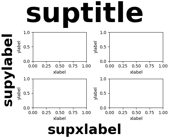
Allow setting figure label size and weight globally and separately from title#
For figure labels, Figure.supxlabel and Figure.supylabel, the size and
weight can be set separately from the figure title using rcParams["figure.labelsize"] (default: 'large')
and rcParams["figure.labelweight"] (default: 'normal').
# Original (previously combined with below) rcParams:
plt.rcParams['figure.titlesize'] = 64
plt.rcParams['figure.titleweight'] = 'bold'

# New rcParams:
plt.rcParams['figure.labelsize'] = 32
plt.rcParams['figure.labelweight'] = 'bold'

fig, axs = plt.subplots(2, 2, layout='constrained')
for ax in axs.flat:
    ax.set(xlabel='xlabel', ylabel='ylabel')

fig.suptitle('suptitle')
fig.supxlabel('supxlabel')
fig.supylabel('supylabel')
(Source code, png)

Note that if you have changed rcParams["figure.titlesize"] (default: 'large') or
rcParams["figure.titleweight"] (default: 'normal'), you must now also change the introduced parameters
for a result consistent with past behaviour.
Mathtext parsing can be disabled globally#
The rcParams["text.parse_math"] (default: True) setting may be used to disable parsing of mathtext in
all Text objects (most notably from the Axes.text method).
Double-quoted strings in matplotlibrc#
You can now use double-quotes around strings. This allows using the '#' character in strings. Without quotes, '#' is interpreted as start of a comment. In particular, you can now define hex-colors:
grid.color: "#b0b0b0"
3D Axes improvements#
Standardized views for primary plane viewing angles#
When viewing a 3D plot in one of the primary view planes (i.e., perpendicular to the XY, XZ, or YZ planes), the Axis will be displayed in a standard location. For further information on 3D views, see mplot3d View Angles and Primary 3D view planes.
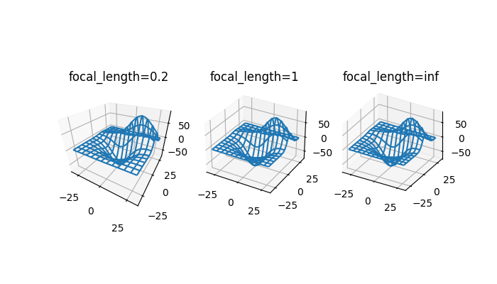
Custom focal length for 3D camera#
The 3D Axes can now better mimic real-world cameras by specifying the focal length of the virtual camera. The default focal length of 1 corresponds to a Field of View (FOV) of 90°, and is backwards-compatible with existing 3D plots. An increased focal length between 1 and infinity "flattens" the image, while a decreased focal length between 1 and 0 exaggerates the perspective and gives the image more apparent depth.
The focal length can be calculated from a desired FOV via the equation:

from mpl_toolkits.mplot3d import axes3d

X, Y, Z = axes3d.get_test_data(0.05)

fig, axs = plt.subplots(1, 3, figsize=(7, 4),
                        subplot_kw={'projection': '3d'})

for ax, focal_length in zip(axs, [0.2, 1, np.inf]):
    ax.plot_wireframe(X, Y, Z, rstride=10, cstride=10)
    ax.set_proj_type('persp', focal_length=focal_length)
    ax.set_title(f"{focal_length=}")
(Source code, png)

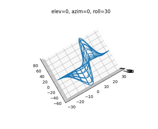
3D plots gained a 3rd "roll" viewing angle#
3D plots can now be viewed from any orientation with the addition of a 3rd roll angle, which rotates the plot about the viewing axis. Interactive rotation using the mouse still only controls elevation and azimuth, meaning that this feature is relevant to users who create more complex camera angles programmatically. The default roll angle of 0 is backwards-compatible with existing 3D plots.
from mpl_toolkits.mplot3d import axes3d

X, Y, Z = axes3d.get_test_data(0.05)

fig, ax = plt.subplots(subplot_kw={'projection': '3d'})

ax.plot_wireframe(X, Y, Z, rstride=10, cstride=10)
ax.view_init(elev=0, azim=0, roll=30)
ax.set_title('elev=0, azim=0, roll=30')
(Source code, png)
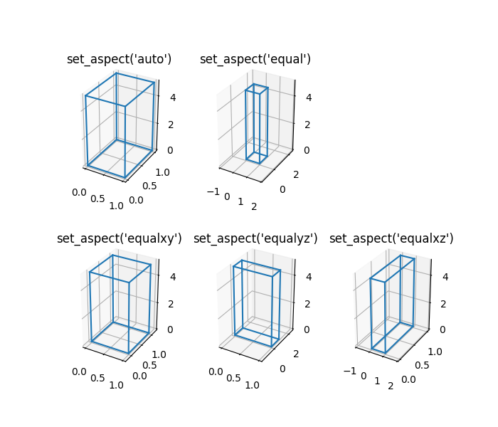
Equal aspect ratio for 3D plots#
Users can set the aspect ratio for the X, Y, Z axes of a 3D plot to be 'equal', 'equalxy', 'equalxz', or 'equalyz' rather than the default of 'auto'.
from itertools import combinations, product

aspects = [
    ['auto', 'equal', '.'],
    ['equalxy', 'equalyz', 'equalxz'],
]
fig, axs = plt.subplot_mosaic(aspects, figsize=(7, 6),
                              subplot_kw={'projection': '3d'})

# Draw rectangular cuboid with side lengths [1, 1, 5]
r = [0, 1]
scale = np.array([1, 1, 5])
pts = combinations(np.array(list(product(r, r, r))), 2)
for start, end in pts:
    if np.sum(np.abs(start - end)) == r[1] - r[0]:
        for ax in axs.values():
            ax.plot3D(*zip(start*scale, end*scale), color='C0')

# Set the aspect ratios
for aspect, ax in axs.items():
    ax.set_box_aspect((3, 4, 5))
    ax.set_aspect(aspect)
    ax.set_title(f'set_aspect({aspect!r})')
(Source code, png)
Interactive tool improvements#
Rotation, aspect ratio correction and add/remove state#
The RectangleSelector and EllipseSelector can now be rotated
interactively between -45° and 45°. The range limits are currently dictated by
the implementation. The rotation is enabled or disabled by striking the r key
('r' is the default key mapped to 'rotate' in state_modifier_keys) or by
calling selector.add_state('rotate').
The aspect ratio of the axes can now be taken into account when using the
"square" state. This is enabled by specifying use_data_coordinates='True'
when the selector is initialized.
In addition to changing selector state interactively using the modifier keys defined in state_modifier_keys, the selector state can now be changed programmatically using the add_state and remove_state methods.
from matplotlib.widgets import RectangleSelector

values = np.arange(0, 100)

fig = plt.figure()
ax = fig.add_subplot()
ax.plot(values, values)

selector = RectangleSelector(ax, print, interactive=True,
                             drag_from_anywhere=True,
                             use_data_coordinates=True)
selector.add_state('rotate')  # alternatively press 'r' key
# rotate the selector interactively

selector.remove_state('rotate')  # alternatively press 'r' key

selector.add_state('square')
MultiCursor now supports Axes split over multiple figures#
Previously, MultiCursor only worked if all target Axes belonged to the same
figure.
As a consequence of this change, the first argument to the MultiCursor
constructor has become unused (it was previously the joint canvas of all Axes,
but the canvases are now directly inferred from the list of Axes).
PolygonSelector bounding boxes#
PolygonSelector now has a draw_bounding_box argument, which when set to
True will draw a bounding box around the polygon once it is complete. The
bounding box can be resized and moved, allowing the points of the polygon to be
easily resized.
Setting PolygonSelector vertices#
The vertices of PolygonSelector can now be set programmatically by using the
PolygonSelector.verts property. Setting the vertices this way will reset the
selector, and create a new complete selector with the supplied vertices.
SpanSelector widget can now be snapped to specified values#
The SpanSelector widget can now be snapped to values specified by the
snap_values argument.
More toolbar icons are styled for dark themes#
On the macOS and Tk backends, toolbar icons will now be inverted when using a dark theme.
Platform-specific changes#
Wx backend uses standard toolbar#
Instead of a custom sizer, the toolbar is set on Wx windows as a standard toolbar.
Improvements to macosx backend#
Modifier keys handled more consistently#
The macosx backend now handles modifier keys in a manner more consistent with other backends. See the table in Event connections for further information.
savefig.directory rcParam support#
The macosx backend will now obey the rcParams["savefig.directory"] (default: '~') setting. If set to
a non-empty string, then the save dialog will default to this directory, and
preserve subsequent save directories as they are changed.
figure.raise_window rcParam support#
The macosx backend will now obey the rcParams["figure.raise_window"] (default: True) setting. If set
to False, figure windows will not be raised to the top on update.
Full-screen toggle support#
As supported on other backends, the macosx backend now supports toggling fullscreen view. By default, this view can be toggled by pressing the f key.
Improved animation and blitting support#
The macosx backend has been improved to fix blitting, animation frames with new artists, and to reduce unnecessary draw calls.
macOS application icon applied on Qt backend#
When using the Qt-based backends on macOS, the application icon will now be set, as is done on other backends/platforms.
New minimum macOS version#
The macosx backend now requires macOS >= 10.12.
Windows on ARM support#
Preliminary support for Windows on arm64 target has been added. This support requires FreeType 2.11 or above.
No binary wheels are available yet but it may be built from source.