Note
Click here to download the full example code
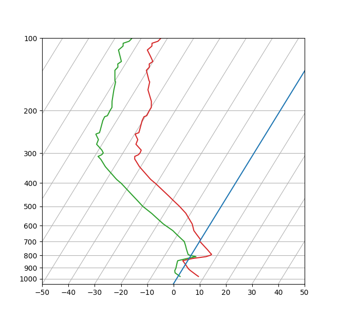
SkewT-logP diagram: using transforms and custom projections#
This serves as an intensive exercise of Matplotlib's transforms and custom projection API. This example produces a so-called SkewT-logP diagram, which is a common plot in meteorology for displaying vertical profiles of temperature. As far as Matplotlib is concerned, the complexity comes from having X and Y axes that are not orthogonal. This is handled by including a skew component to the basic Axes transforms. Additional complexity comes in handling the fact that the upper and lower X-axes have different data ranges, which necessitates a bunch of custom classes for ticks, spines, and axis to handle this.
from contextlib import ExitStack

from matplotlib.axes import Axes
import matplotlib.transforms as transforms
import matplotlib.axis as maxis
import matplotlib.spines as mspines
from matplotlib.projections import register_projection


# The sole purpose of this class is to look at the upper, lower, or total
# interval as appropriate and see what parts of the tick to draw, if any.
class SkewXTick(maxis.XTick):
    def draw(self, renderer):
        # When adding the callbacks with `stack.callback`, we fetch the current
        # visibility state of the artist with `get_visible`; the ExitStack will
        # restore these states (`set_visible`) at the end of the block (after
        # the draw).
        with ExitStack() as stack:
            for artist in [self.gridline, self.tick1line, self.tick2line,
                           self.label1, self.label2]:
                stack.callback(artist.set_visible, artist.get_visible())
            needs_lower = transforms.interval_contains(
                self.axes.lower_xlim, self.get_loc())
            needs_upper = transforms.interval_contains(
                self.axes.upper_xlim, self.get_loc())
            self.tick1line.set_visible(
                self.tick1line.get_visible() and needs_lower)
            self.label1.set_visible(
                self.label1.get_visible() and needs_lower)
            self.tick2line.set_visible(
                self.tick2line.get_visible() and needs_upper)
            self.label2.set_visible(
                self.label2.get_visible() and needs_upper)
            super().draw(renderer)

    def get_view_interval(self):
        return self.axes.xaxis.get_view_interval()


# This class exists to provide two separate sets of intervals to the tick,
# as well as create instances of the custom tick
class SkewXAxis(maxis.XAxis):
    def _get_tick(self, major):
        return SkewXTick(self.axes, None, major=major)

    def get_view_interval(self):
        return self.axes.upper_xlim[0], self.axes.lower_xlim[1]


# This class exists to calculate the separate data range of the
# upper X-axis and draw the spine there. It also provides this range
# to the X-axis artist for ticking and gridlines
class SkewSpine(mspines.Spine):
    def _adjust_location(self):
        pts = self._path.vertices
        if self.spine_type == 'top':
            pts[:, 0] = self.axes.upper_xlim
        else:
            pts[:, 0] = self.axes.lower_xlim


# This class handles registration of the skew-xaxes as a projection as well
# as setting up the appropriate transformations. It also overrides standard
# spines and axes instances as appropriate.
class SkewXAxes(Axes):
    # The projection must specify a name.  This will be used be the
    # user to select the projection, i.e. ``subplot(projection='skewx')``.
    name = 'skewx'

    def _init_axis(self):
        # Taken from Axes and modified to use our modified X-axis
        self.xaxis = SkewXAxis(self)
        self.spines.top.register_axis(self.xaxis)
        self.spines.bottom.register_axis(self.xaxis)
        self.yaxis = maxis.YAxis(self)
        self.spines.left.register_axis(self.yaxis)
        self.spines.right.register_axis(self.yaxis)

    def _gen_axes_spines(self):
        spines = {'top': SkewSpine.linear_spine(self, 'top'),
                  'bottom': mspines.Spine.linear_spine(self, 'bottom'),
                  'left': mspines.Spine.linear_spine(self, 'left'),
                  'right': mspines.Spine.linear_spine(self, 'right')}
        return spines

    def _set_lim_and_transforms(self):
        """
        This is called once when the plot is created to set up all the
        transforms for the data, text and grids.
        """
        rot = 30

        # Get the standard transform setup from the Axes base class
        super()._set_lim_and_transforms()

        # Need to put the skew in the middle, after the scale and limits,
        # but before the transAxes. This way, the skew is done in Axes
        # coordinates thus performing the transform around the proper origin
        # We keep the pre-transAxes transform around for other users, like the
        # spines for finding bounds
        self.transDataToAxes = (
            self.transScale
            + self.transLimits
            + transforms.Affine2D().skew_deg(rot, 0)
        )
        # Create the full transform from Data to Pixels
        self.transData = self.transDataToAxes + self.transAxes

        # Blended transforms like this need to have the skewing applied using
        # both axes, in axes coords like before.
        self._xaxis_transform = (
            transforms.blended_transform_factory(
                self.transScale + self.transLimits,
                transforms.IdentityTransform())
            + transforms.Affine2D().skew_deg(rot, 0)
            + self.transAxes
        )

    @property
    def lower_xlim(self):
        return self.axes.viewLim.intervalx

    @property
    def upper_xlim(self):
        pts = [[0., 1.], [1., 1.]]
        return self.transDataToAxes.inverted().transform(pts)[:, 0]


# Now register the projection with matplotlib so the user can select it.
register_projection(SkewXAxes)

if __name__ == '__main__':
    # Now make a simple example using the custom projection.
    from io import StringIO
    from matplotlib.ticker import (MultipleLocator, NullFormatter,
                                   ScalarFormatter)
    import matplotlib.pyplot as plt
    import numpy as np

    # Some example data.
    data_txt = '''
        978.0    345    7.8    0.8
        971.0    404    7.2    0.2
        946.7    610    5.2   -1.8
        944.0    634    5.0   -2.0
        925.0    798    3.4   -2.6
        911.8    914    2.4   -2.7
        906.0    966    2.0   -2.7
        877.9   1219    0.4   -3.2
        850.0   1478   -1.3   -3.7
        841.0   1563   -1.9   -3.8
        823.0   1736    1.4   -0.7
        813.6   1829    4.5    1.2
        809.0   1875    6.0    2.2
        798.0   1988    7.4   -0.6
        791.0   2061    7.6   -1.4
        783.9   2134    7.0   -1.7
        755.1   2438    4.8   -3.1
        727.3   2743    2.5   -4.4
        700.5   3048    0.2   -5.8
        700.0   3054    0.2   -5.8
        698.0   3077    0.0   -6.0
        687.0   3204   -0.1   -7.1
        648.9   3658   -3.2  -10.9
        631.0   3881   -4.7  -12.7
        600.7   4267   -6.4  -16.7
        592.0   4381   -6.9  -17.9
        577.6   4572   -8.1  -19.6
        555.3   4877  -10.0  -22.3
        536.0   5151  -11.7  -24.7
        533.8   5182  -11.9  -25.0
        500.0   5680  -15.9  -29.9
        472.3   6096  -19.7  -33.4
        453.0   6401  -22.4  -36.0
        400.0   7310  -30.7  -43.7
        399.7   7315  -30.8  -43.8
        387.0   7543  -33.1  -46.1
        382.7   7620  -33.8  -46.8
        342.0   8398  -40.5  -53.5
        320.4   8839  -43.7  -56.7
        318.0   8890  -44.1  -57.1
        310.0   9060  -44.7  -58.7
        306.1   9144  -43.9  -57.9
        305.0   9169  -43.7  -57.7
        300.0   9280  -43.5  -57.5
        292.0   9462  -43.7  -58.7
        276.0   9838  -47.1  -62.1
        264.0  10132  -47.5  -62.5
        251.0  10464  -49.7  -64.7
        250.0  10490  -49.7  -64.7
        247.0  10569  -48.7  -63.7
        244.0  10649  -48.9  -63.9
        243.3  10668  -48.9  -63.9
        220.0  11327  -50.3  -65.3
        212.0  11569  -50.5  -65.5
        210.0  11631  -49.7  -64.7
        200.0  11950  -49.9  -64.9
        194.0  12149  -49.9  -64.9
        183.0  12529  -51.3  -66.3
        164.0  13233  -55.3  -68.3
        152.0  13716  -56.5  -69.5
        150.0  13800  -57.1  -70.1
        136.0  14414  -60.5  -72.5
        132.0  14600  -60.1  -72.1
        131.4  14630  -60.2  -72.2
        128.0  14792  -60.9  -72.9
        125.0  14939  -60.1  -72.1
        119.0  15240  -62.2  -73.8
        112.0  15616  -64.9  -75.9
        108.0  15838  -64.1  -75.1
        107.8  15850  -64.1  -75.1
        105.0  16010  -64.7  -75.7
        103.0  16128  -62.9  -73.9
        100.0  16310  -62.5  -73.5
    '''

    # Parse the data
    sound_data = StringIO(data_txt)
    p, h, T, Td = np.loadtxt(sound_data, unpack=True)

    # Create a new figure. The dimensions here give a good aspect ratio
    fig = plt.figure(figsize=(6.5875, 6.2125))
    ax = fig.add_subplot(projection='skewx')

    plt.grid(True)

    # Plot the data using normal plotting functions, in this case using
    # log scaling in Y, as dictated by the typical meteorological plot
    ax.semilogy(T, p, color='C3')
    ax.semilogy(Td, p, color='C2')

    # An example of a slanted line at constant X
    l = ax.axvline(0, color='C0')

    # Disables the log-formatting that comes with semilogy
    ax.yaxis.set_major_formatter(ScalarFormatter())
    ax.yaxis.set_minor_formatter(NullFormatter())
    ax.set_yticks(np.linspace(100, 1000, 10))
    ax.set_ylim(1050, 100)

    ax.xaxis.set_major_locator(MultipleLocator(10))
    ax.set_xlim(-50, 50)

    plt.show()
References
The use of the following functions, methods, classes and modules is shown in this example: