Note
Click here to download the full example code
Arranging multiple Axes in a Figure#
Often more than one Axes is wanted on a figure at a time, usually organized into a regular grid. Matplotlib has a variety of tools for working with grids of Axes that have evolved over the history of the library. Here we will discuss the tools we think users should use most often, the tools that underpin how Axes are organized, and mention some of the older tools.
Note
Matplotlib uses Axes to refer to the drawing area that contains data, x- and y-axis, ticks, labels, title, etc. See Parts of a Figure for more details. Another term that is often used is "subplot", which refers to an Axes that is in a grid with other Axes objects.
Overview#
Create grid-shaped combinations of Axes#
subplotsThe primary function used to create figures and a grid of Axes. It creates and places all Axes on the figure at once, and returns an object array with handles for the Axes in the grid. See
Figure.subplots.
or
subplot_mosaicA simple way to create figures and a grid of Axes, with the added flexibility that Axes can also span rows or columns. The Axes are returned in a labelled dictionary instead of an array. See also
Figure.subplot_mosaicand Complex and semantic figure composition.
Sometimes it is natural to have more than one distinct group of Axes grids,
in which case Matplotlib has the concept of SubFigure:
SubFigureA virtual figure within a figure.
Underlying tools#
Underlying these are the concept of a GridSpec and
a SubplotSpec:
GridSpecSpecifies the geometry of the grid that a subplot will be placed. The number of rows and number of columns of the grid need to be set. Optionally, the subplot layout parameters (e.g., left, right, etc.) can be tuned.
SubplotSpecSpecifies the location of the subplot in the given
GridSpec.
Adding single Axes at a time#
The above functions create all Axes in a single function call. It is also possible to add Axes one at a time, and this was originally how Matplotlib used to work. Doing so is generally less elegant and flexible, though sometimes useful for interactive work or to place an Axes in a custom location:
add_axesAdds a single axes at a location specified by
[left, bottom, width, height]in fractions of figure width or height.subplotorFigure.add_subplotAdds a single subplot on a figure, with 1-based indexing (inherited from Matlab). Columns and rows can be spanned by specifying a range of grid cells.
subplot2gridSimilar to
pyplot.subplot, but uses 0-based indexing and two-d python slicing to choose cells.
High-level methods for making grids#
Basic 2x2 grid#
We can create a basic 2-by-2 grid of Axes using
subplots. It returns a Figure
instance and an array of Axes objects. The Axes
objects can be used to access methods to place artists on the Axes; here
we use annotate, but other examples could be plot,
pcolormesh, etc.
import matplotlib.pyplot as plt
import numpy as np

fig, axs = plt.subplots(ncols=2, nrows=2, figsize=(5.5, 3.5),
                        constrained_layout=True)
# add an artist, in this case a nice label in the middle...
for row in range(2):
    for col in range(2):
        axs[row, col].annotate(f'axs[{row}, {col}]', (0.5, 0.5),
                               transform=axs[row, col].transAxes,
                               ha='center', va='center', fontsize=18,
                               color='darkgrey')
fig.suptitle('plt.subplots()')
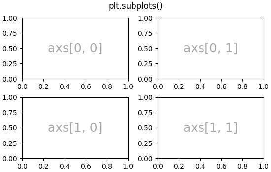
Text(0.5, 0.9880942857142857, 'plt.subplots()')
We will annotate a lot of Axes, so lets encapsulate the annotation, rather than having that large piece of annotation code every time we need it:
def annotate_axes(ax, text, fontsize=18):
    ax.text(0.5, 0.5, text, transform=ax.transAxes,
            ha="center", va="center", fontsize=fontsize, color="darkgrey")
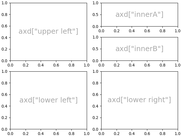
The same effect can be achieved with subplot_mosaic,
but the return type is a dictionary instead of an array, where the user
can give the keys useful meanings. Here we provide two lists, each list
representing a row, and each element in the list a key representing the
column.
fig, axd = plt.subplot_mosaic([['upper left', 'upper right'],
                               ['lower left', 'lower right']],
                              figsize=(5.5, 3.5), constrained_layout=True)
for k in axd:
    annotate_axes(axd[k], f'axd["{k}"]', fontsize=14)
fig.suptitle('plt.subplot_mosaic()')
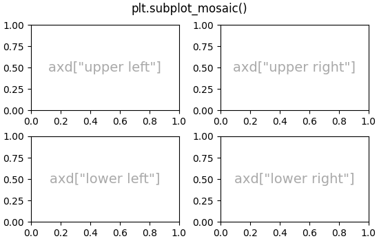
Text(0.5, 0.9880942857142857, 'plt.subplot_mosaic()')
Axes spanning rows or columns in a grid#
Sometimes we want Axes to span rows or columns of the grid.
There are actually multiple ways to accomplish this, but the most
convenient is probably to use subplot_mosaic by repeating one
of the keys:
fig, axd = plt.subplot_mosaic([['upper left', 'right'],
                               ['lower left', 'right']],
                              figsize=(5.5, 3.5), constrained_layout=True)
for k in axd:
    annotate_axes(axd[k], f'axd["{k}"]', fontsize=14)
fig.suptitle('plt.subplot_mosaic()')
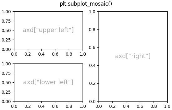
Text(0.5, 0.9880942857142857, 'plt.subplot_mosaic()')
See below for the description of how to do the same thing using
GridSpec or subplot2grid.
Variable widths or heights in a grid#
Both subplots and subplot_mosaic allow the rows
in the grid to be different heights, and the columns to be different
widths using the gridspec_kw keyword argument.
Spacing parameters accepted by GridSpec
can be passed to subplots and
subplot_mosaic:
gs_kw = dict(width_ratios=[1.4, 1], height_ratios=[1, 2])
fig, axd = plt.subplot_mosaic([['upper left', 'right'],
                               ['lower left', 'right']],
                              gridspec_kw=gs_kw, figsize=(5.5, 3.5),
                              constrained_layout=True)
for k in axd:
    annotate_axes(axd[k], f'axd["{k}"]', fontsize=14)
fig.suptitle('plt.subplot_mosaic()')
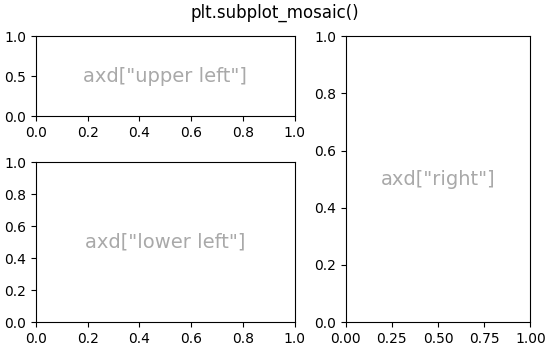
Text(0.5, 0.9880942857142857, 'plt.subplot_mosaic()')
Nested Axes layouts#
Sometimes it is helpful to have two or more grids of Axes that
may not need to be related to one another. The most simple way to
accomplish this is to use Figure.subfigures. Note that the subfigure
layouts are independent, so the Axes spines in each subfigure are not
necessarily aligned. See below for a more verbose way to achieve the same
effect with GridSpecFromSubplotSpec.
fig = plt.figure(constrained_layout=True)
subfigs = fig.subfigures(1, 2, wspace=0.07, width_ratios=[1.5, 1.])
axs0 = subfigs[0].subplots(2, 2)
subfigs[0].set_facecolor('0.9')
subfigs[0].suptitle('subfigs[0]\nLeft side')
subfigs[0].supxlabel('xlabel for subfigs[0]')

axs1 = subfigs[1].subplots(3, 1)
subfigs[1].suptitle('subfigs[1]')
subfigs[1].supylabel('ylabel for subfigs[1]')
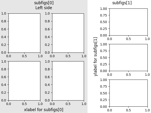
Text(0.016867713730569944, 0.5, 'ylabel for subfigs[1]')
It is also possible to nest Axes using subplot_mosaic using
nested lists. This method does not use subfigures, like above, so lacks
the ability to add per-subfigure suptitle and supxlabel, etc.
Rather it is a convenience wrapper around the subgridspec
method described below.
Low-level and advanced grid methods#
Internally, the arrangement of a grid of Axes is controlled by creating
instances of GridSpec and SubplotSpec. GridSpec defines a
(possibly non-uniform) grid of cells. Indexing into the GridSpec returns
a SubplotSpec that covers one or more grid cells, and can be used to
specify the location of an Axes.
The following examples show how to use low-level methods to arrange Axes using GridSpec objects.
Basic 2x2 grid#
We can accopmplish a 2x2 grid in the same manner as
plt.subplots(2, 2):
fig = plt.figure(figsize=(5.5, 3.5), constrained_layout=True)
spec = fig.add_gridspec(ncols=2, nrows=2)

ax0 = fig.add_subplot(spec[0, 0])
annotate_axes(ax0, 'ax0')

ax1 = fig.add_subplot(spec[0, 1])
annotate_axes(ax1, 'ax1')

ax2 = fig.add_subplot(spec[1, 0])
annotate_axes(ax2, 'ax2')

ax3 = fig.add_subplot(spec[1, 1])
annotate_axes(ax3, 'ax3')

fig.suptitle('Manually added subplots using add_gridspec')
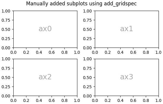
Text(0.5, 0.9880942857142857, 'Manually added subplots using add_gridspec')
Axes spanning rows or grids in a grid#
We can index the spec array using NumPy slice syntax
and the new Axes will span the slice. This would be the same
as fig, axd = plt.subplot_mosaic([['ax0', 'ax0'], ['ax1', 'ax2']], ...):
fig = plt.figure(figsize=(5.5, 3.5), constrained_layout=True)
spec = fig.add_gridspec(2, 2)

ax0 = fig.add_subplot(spec[0, :])
annotate_axes(ax0, 'ax0')

ax10 = fig.add_subplot(spec[1, 0])
annotate_axes(ax10, 'ax10')

ax11 = fig.add_subplot(spec[1, 1])
annotate_axes(ax11, 'ax11')

fig.suptitle('Manually added subplots, spanning a column')
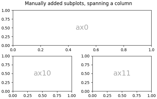
Text(0.5, 0.9880942857142857, 'Manually added subplots, spanning a column')
Manual adjustments to a GridSpec layout#
When a GridSpec is explicitly used, you can adjust the layout
parameters of subplots that are created from the GridSpec. Note this
option is not compatible with constrained_layout or
Figure.tight_layout which both ignore left and right and adjust
subplot sizes to fill the figure. Usually such manual placement
requires iterations to make the Axes tick labels not overlap the Axes.
These spacing parameters can also be passed to subplots and
subplot_mosaic as the gridspec_kw argument.
fig = plt.figure(constrained_layout=False, facecolor='0.9')
gs = fig.add_gridspec(nrows=3, ncols=3, left=0.05, right=0.75,
                      hspace=0.1, wspace=0.05)
ax0 = fig.add_subplot(gs[:-1, :])
annotate_axes(ax0, 'ax0')
ax1 = fig.add_subplot(gs[-1, :-1])
annotate_axes(ax1, 'ax1')
ax2 = fig.add_subplot(gs[-1, -1])
annotate_axes(ax2, 'ax2')
fig.suptitle('Manual gridspec with right=0.75')
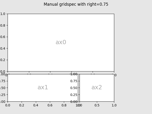
Text(0.5, 0.98, 'Manual gridspec with right=0.75')
Nested layouts with SubplotSpec#
You can create nested layout similar to subfigures using
subgridspec. Here the Axes spines are
aligned.
Note this is also available from the more verbose
gridspec.GridSpecFromSubplotSpec.
fig = plt.figure(constrained_layout=True)
gs0 = fig.add_gridspec(1, 2)

gs00 = gs0[0].subgridspec(2, 2)
gs01 = gs0[1].subgridspec(3, 1)

for a in range(2):
    for b in range(2):
        ax = fig.add_subplot(gs00[a, b])
        annotate_axes(ax, f'axLeft[{a}, {b}]', fontsize=10)
        if a == 1 and b == 1:
            ax.set_xlabel('xlabel')
for a in range(3):
    ax = fig.add_subplot(gs01[a])
    annotate_axes(ax, f'axRight[{a}, {b}]')
    if a == 2:
        ax.set_ylabel('ylabel')

fig.suptitle('nested gridspecs')
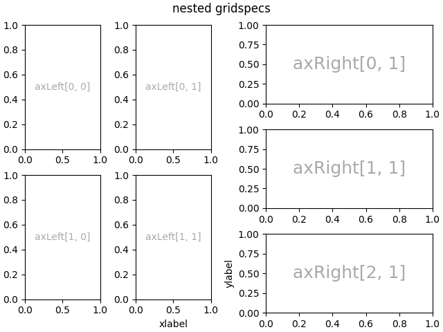
Text(0.5, 0.99131875, 'nested gridspecs')
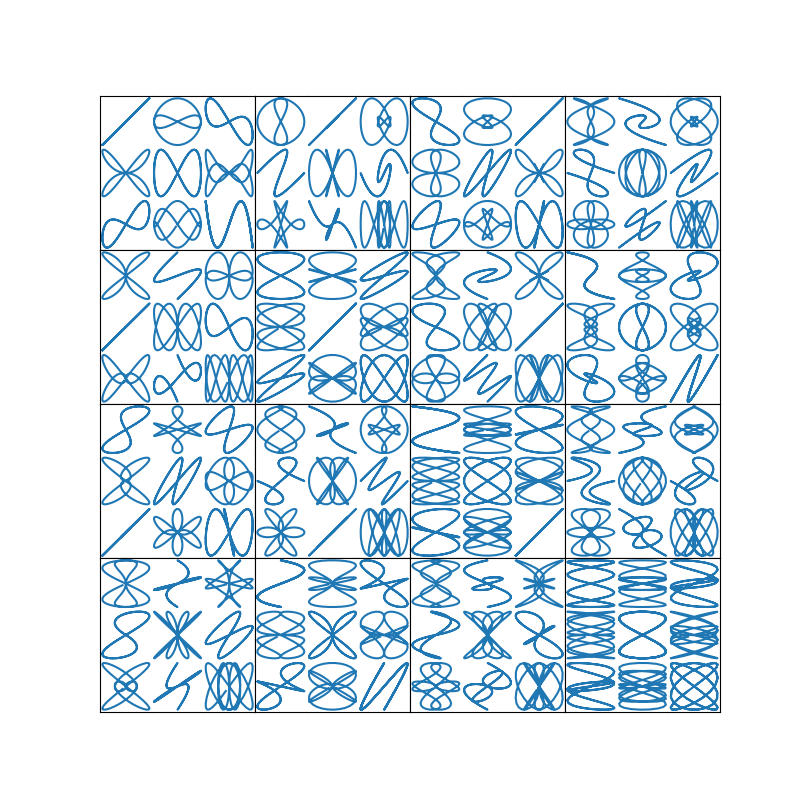
Here's a more sophisticated example of nested GridSpec: We create an outer 4x4 grid with each cell containing an inner 3x3 grid of Axes. We outline the outer 4x4 grid by hiding appropriate spines in each of the inner 3x3 grids.
def squiggle_xy(a, b, c, d, i=np.arange(0.0, 2*np.pi, 0.05)):
    return np.sin(i*a)*np.cos(i*b), np.sin(i*c)*np.cos(i*d)

fig = plt.figure(figsize=(8, 8), constrained_layout=False)
outer_grid = fig.add_gridspec(4, 4, wspace=0, hspace=0)

for a in range(4):
    for b in range(4):
        # gridspec inside gridspec
        inner_grid = outer_grid[a, b].subgridspec(3, 3, wspace=0, hspace=0)
        axs = inner_grid.subplots()  # Create all subplots for the inner grid.
        for (c, d), ax in np.ndenumerate(axs):
            ax.plot(*squiggle_xy(a + 1, b + 1, c + 1, d + 1))
            ax.set(xticks=[], yticks=[])

# show only the outside spines
for ax in fig.get_axes():
    ss = ax.get_subplotspec()
    ax.spines.top.set_visible(ss.is_first_row())
    ax.spines.bottom.set_visible(ss.is_last_row())
    ax.spines.left.set_visible(ss.is_first_col())
    ax.spines.right.set_visible(ss.is_last_col())

plt.show()
More reading#
More details about subplot mosaic.
More details about constrained layout, used to align spacing in most of these examples.
References
The use of the following functions, methods, classes and modules is shown in this example:
Total running time of the script: ( 0 minutes 9.095 seconds)
Keywords: matplotlib code example, codex, python plot, pyplot Gallery generated by Sphinx-Gallery