Note
Click here to download the full example code
The mplot3d Toolkit#
Generating 3D plots using the mplot3d toolkit.
Contents
3D Axes (of class Axes3D) are created by passing the projection="3d"
keyword argument to Figure.add_subplot:
import matplotlib.pyplot as plt
fig = plt.figure()
ax = fig.add_subplot(projection='3d')
Multiple 3D subplots can be added on the same figure, as for 2D subplots.
Changed in version 1.0.0: Prior to Matplotlib 1.0.0, only a single Axes3D could be created per
figure; it needed to be directly instantiated as ax = Axes3D(fig).
Changed in version 3.2.0: Prior to Matplotlib 3.2.0, it was necessary to explicitly import the
mpl_toolkits.mplot3d module to make the '3d' projection to
Figure.add_subplot.
See the mplot3d FAQ for more information about the mplot3d toolkit.
Line plots#
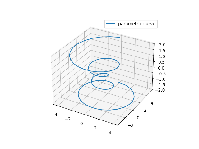
- Axes3D.plot(xs, ys, *args, zdir='z', **kwargs)[source]#
Plot 2D or 3D data.
- Parameters
- xs1D array-like
x coordinates of vertices.
- ys1D array-like
y coordinates of vertices.
- zsfloat or 1D array-like
z coordinates of vertices; either one for all points or one for each point.
- zdir{'x', 'y', 'z'}, default: 'z'
When plotting 2D data, the direction to use as z ('x', 'y' or 'z').
- **kwargs
Other arguments are forwarded to
matplotlib.axes.Axes.plot.
Scatter plots#
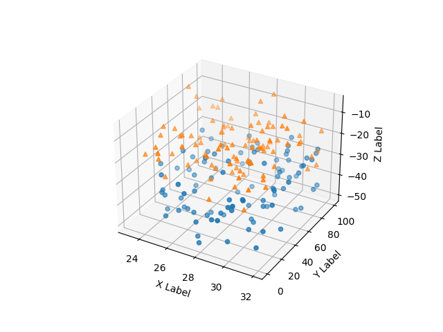
- Axes3D.scatter(xs, ys, zs=0, zdir='z', s=20, c=None, depthshade=True, *args, data=None, **kwargs)[source]#
Create a scatter plot.
- Parameters
- xs, ysarray-like
The data positions.
- zsfloat or array-like, default: 0
The z-positions. Either an array of the same length as xs and ys or a single value to place all points in the same plane.
- zdir{'x', 'y', 'z', '-x', '-y', '-z'}, default: 'z'
The axis direction for the zs. This is useful when plotting 2D data on a 3D Axes. The data must be passed as xs, ys. Setting zdir to 'y' then plots the data to the x-z-plane.
See also Plot 2D data on 3D plot.
- sfloat or array-like, default: 20
The marker size in points**2. Either an array of the same length as xs and ys or a single value to make all markers the same size.
- ccolor, sequence, or sequence of colors, optional
The marker color. Possible values:
A single color format string.
A sequence of colors of length n.
A sequence of n numbers to be mapped to colors using cmap and norm.
A 2D array in which the rows are RGB or RGBA.
For more details see the c argument of
scatter.- depthshadebool, default: True
Whether to shade the scatter markers to give the appearance of depth. Each call to
scatter()will perform its depthshading independently.- dataindexable object, optional
If given, the following parameters also accept a string
s, which is interpreted asdata[s](unless this raises an exception):xs, ys, zs, s, edgecolors, c, facecolor, facecolors, color
- **kwargs
All other arguments are passed on to
scatter.
- Returns
- paths
PathCollection
- paths
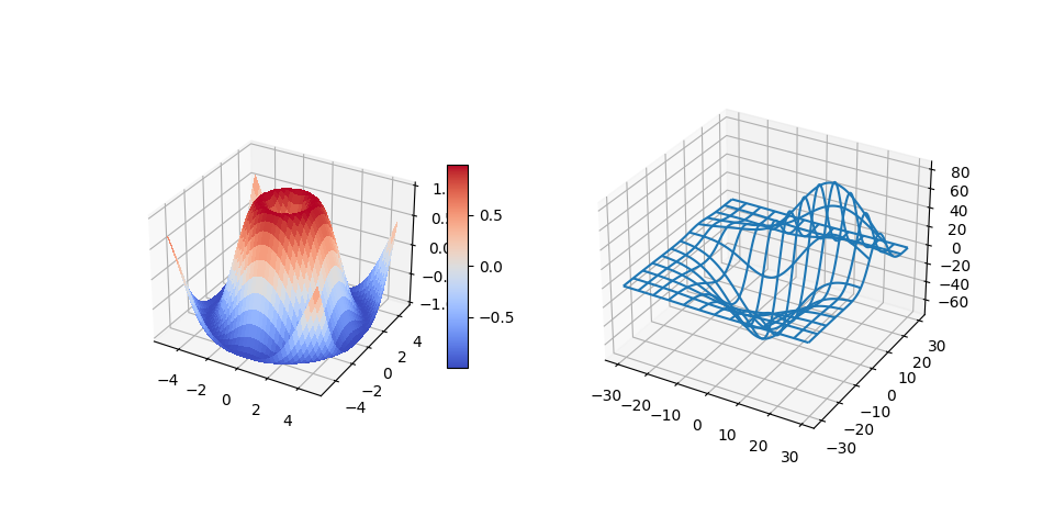
Wireframe plots#
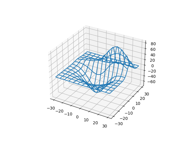
- Axes3D.plot_wireframe(X, Y, Z, *args, **kwargs)[source]#
Plot a 3D wireframe.
Note
The rcount and ccount kwargs, which both default to 50, determine the maximum number of samples used in each direction. If the input data is larger, it will be downsampled (by slicing) to these numbers of points.
- Parameters
- X, Y, Z2D arrays
Data values.
- rcount, ccountint
Maximum number of samples used in each direction. If the input data is larger, it will be downsampled (by slicing) to these numbers of points. Setting a count to zero causes the data to be not sampled in the corresponding direction, producing a 3D line plot rather than a wireframe plot. Defaults to 50.
- rstride, cstrideint
Downsampling stride in each direction. These arguments are mutually exclusive with rcount and ccount. If only one of rstride or cstride is set, the other defaults to 1. Setting a stride to zero causes the data to be not sampled in the corresponding direction, producing a 3D line plot rather than a wireframe plot.
'classic' mode uses a default of
rstride = cstride = 1instead of the new default ofrcount = ccount = 50.- **kwargs
Other arguments are forwarded to
Line3DCollection.
Surface plots#
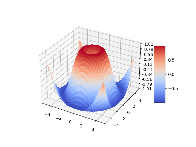
- Axes3D.plot_surface(X, Y, Z, *args, norm=None, vmin=None, vmax=None, lightsource=None, **kwargs)[source]#
Create a surface plot.
By default it will be colored in shades of a solid color, but it also supports colormapping by supplying the cmap argument.
Note
The rcount and ccount kwargs, which both default to 50, determine the maximum number of samples used in each direction. If the input data is larger, it will be downsampled (by slicing) to these numbers of points.
Note
To maximize rendering speed consider setting rstride and cstride to divisors of the number of rows minus 1 and columns minus 1 respectively. For example, given 51 rows rstride can be any of the divisors of 50.
Similarly, a setting of rstride and cstride equal to 1 (or rcount and ccount equal the number of rows and columns) can use the optimized path.
- Parameters
- X, Y, Z2D arrays
Data values.
- rcount, ccountint
Maximum number of samples used in each direction. If the input data is larger, it will be downsampled (by slicing) to these numbers of points. Defaults to 50.
- rstride, cstrideint
Downsampling stride in each direction. These arguments are mutually exclusive with rcount and ccount. If only one of rstride or cstride is set, the other defaults to 10.
'classic' mode uses a default of
rstride = cstride = 10instead of the new default ofrcount = ccount = 50.- colorcolor-like
Color of the surface patches.
- cmapColormap
Colormap of the surface patches.
- facecolorsarray-like of colors.
Colors of each individual patch.
- normNormalize
Normalization for the colormap.
- vmin, vmaxfloat
Bounds for the normalization.
- shadebool, default: True
Whether to shade the facecolors. Shading is always disabled when cmap is specified.
- lightsource
LightSource The lightsource to use when shade is True.
- **kwargs
Other arguments are forwarded to
Poly3DCollection.
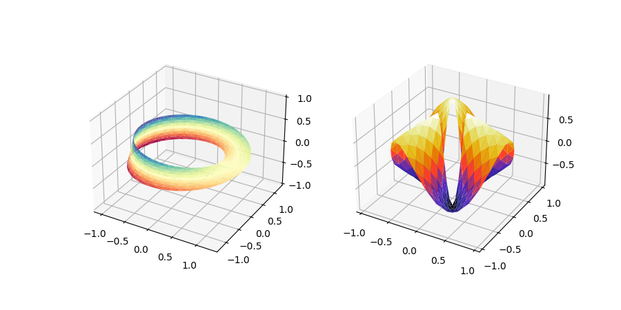
Tri-Surface plots#
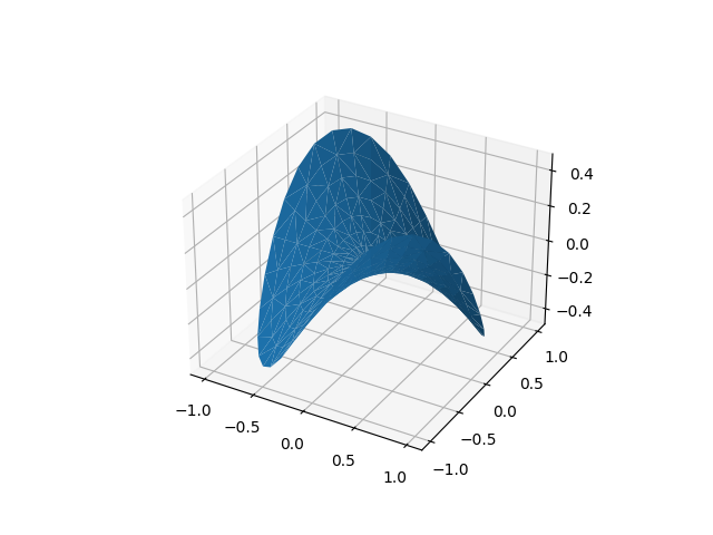
- Axes3D.plot_trisurf(*args, color=None, norm=None, vmin=None, vmax=None, lightsource=None, **kwargs)[source]#
Plot a triangulated surface.
The (optional) triangulation can be specified in one of two ways; either:
plot_trisurf(triangulation, ...)
where triangulation is a
Triangulationobject, or:plot_trisurf(X, Y, ...) plot_trisurf(X, Y, triangles, ...) plot_trisurf(X, Y, triangles=triangles, ...)
in which case a Triangulation object will be created. See
Triangulationfor a explanation of these possibilities.The remaining arguments are:
plot_trisurf(..., Z)
where Z is the array of values to contour, one per point in the triangulation.
- Parameters
- X, Y, Zarray-like
Data values as 1D arrays.
- color
Color of the surface patches.
- cmap
A colormap for the surface patches.
- normNormalize
An instance of Normalize to map values to colors.
- vmin, vmaxfloat, default: None
Minimum and maximum value to map.
- shadebool, default: True
Whether to shade the facecolors. Shading is always disabled when cmap is specified.
- lightsource
LightSource The lightsource to use when shade is True.
- **kwargs
All other arguments are passed on to
Poly3DCollection
Examples
(Source code, png, pdf)
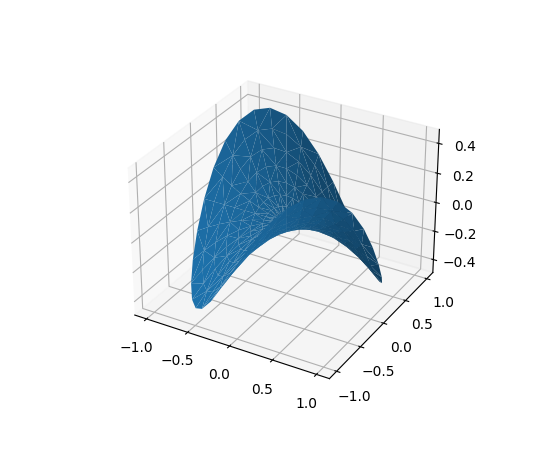
(Source code, png, pdf)
Contour plots#
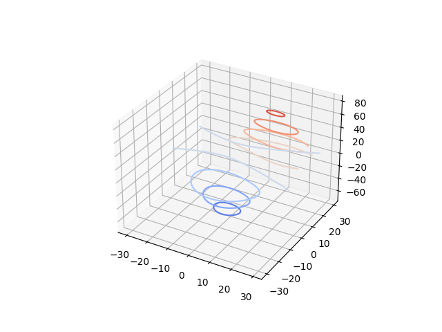
- Axes3D.contour(X, Y, Z, *args, extend3d=False, stride=5, zdir='z', offset=None, data=None, **kwargs)[source]#
Create a 3D contour plot.
- Parameters
- X, Y, Zarray-like,
Input data. See
contourfor acceptable data shapes.- extend3dbool, default: False
Whether to extend contour in 3D.
- strideint
Step size for extending contour.
- zdir{'x', 'y', 'z'}, default: 'z'
The direction to use.
- offsetfloat, optional
If specified, plot a projection of the contour lines at this position in a plane normal to zdir.
- dataindexable object, optional
If given, all parameters also accept a string
s, which is interpreted asdata[s](unless this raises an exception).- *args, **kwargs
Other arguments are forwarded to
matplotlib.axes.Axes.contour.
- Returns
- matplotlib.contour.QuadContourSet
Filled contour plots#
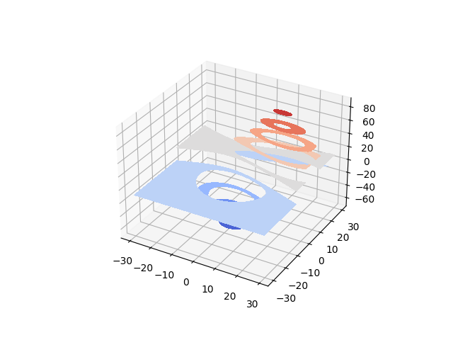
- Axes3D.contourf(X, Y, Z, *args, zdir='z', offset=None, data=None, **kwargs)[source]#
Create a 3D filled contour plot.
- Parameters
- X, Y, Zarray-like
Input data. See
contourffor acceptable data shapes.- zdir{'x', 'y', 'z'}, default: 'z'
The direction to use.
- offsetfloat, optional
If specified, plot a projection of the contour lines at this position in a plane normal to zdir.
- dataindexable object, optional
If given, all parameters also accept a string
s, which is interpreted asdata[s](unless this raises an exception).- *args, **kwargs
Other arguments are forwarded to
matplotlib.axes.Axes.contourf.
- Returns
- matplotlib.contour.QuadContourSet
New in version 1.1.0: The feature demoed in the second contourf3d example was enabled as a result of a bugfix for version 1.1.0.
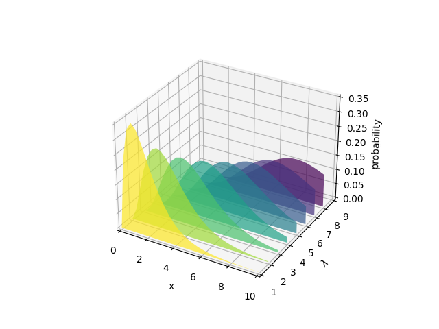
Polygon plots#
Bar plots#
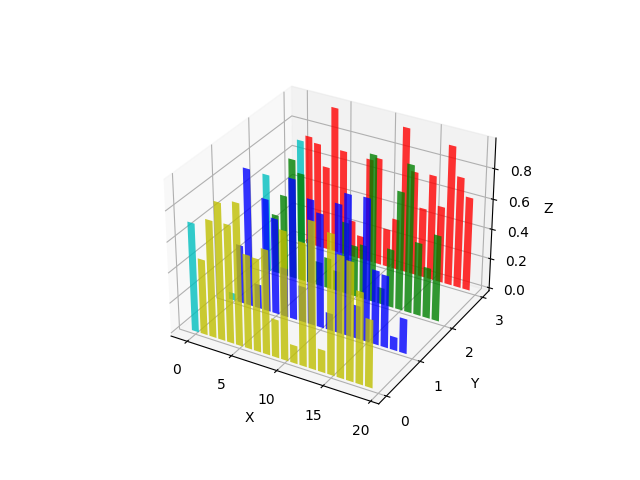
- Axes3D.bar(left, height, zs=0, zdir='z', *args, data=None, **kwargs)[source]#
Add 2D bar(s).
- Parameters
- left1D array-like
The x coordinates of the left sides of the bars.
- height1D array-like
The height of the bars.
- zsfloat or 1D array-like
Z coordinate of bars; if a single value is specified, it will be used for all bars.
- zdir{'x', 'y', 'z'}, default: 'z'
When plotting 2D data, the direction to use as z ('x', 'y' or 'z').
- dataindexable object, optional
If given, all parameters also accept a string
s, which is interpreted asdata[s](unless this raises an exception).- **kwargs
Other arguments are forwarded to
matplotlib.axes.Axes.bar.
- Returns
- mpl_toolkits.mplot3d.art3d.Patch3DCollection
Quiver#
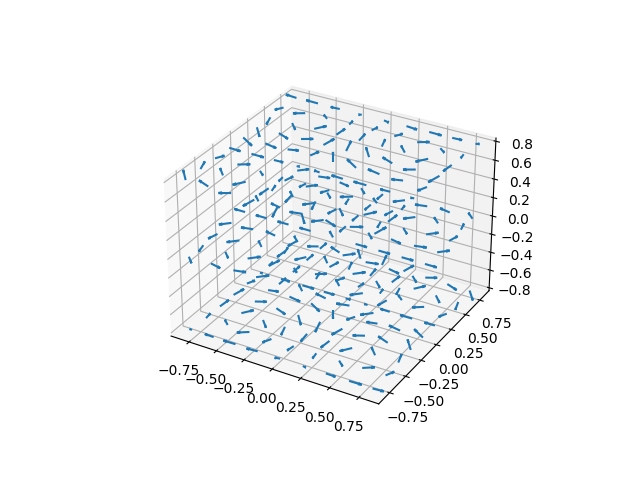
- Axes3D.quiver(X, Y, Z, U, V, W, /, length=1, arrow_length_ratio=.3, pivot='tail', normalize=False, **kwargs)[source]#
Plot a 3D field of arrows.
The arguments could be array-like or scalars, so long as they they can be broadcast together. The arguments can also be masked arrays. If an element in any of argument is masked, then that corresponding quiver element will not be plotted.
- Parameters
- X, Y, Zarray-like
The x, y and z coordinates of the arrow locations (default is tail of arrow; see pivot kwarg).
- U, V, Warray-like
The x, y and z components of the arrow vectors.
- lengthfloat, default: 1
The length of each quiver.
- arrow_length_ratiofloat, default: 0.3
The ratio of the arrow head with respect to the quiver.
- pivot{'tail', 'middle', 'tip'}, default: 'tail'
The part of the arrow that is at the grid point; the arrow rotates about this point, hence the name pivot.
- normalizebool, default: False
Whether all arrows are normalized to have the same length, or keep the lengths defined by u, v, and w.
- dataindexable object, optional
If given, all parameters also accept a string
s, which is interpreted asdata[s](unless this raises an exception).- **kwargs
Any additional keyword arguments are delegated to
LineCollection
2D plots in 3D#
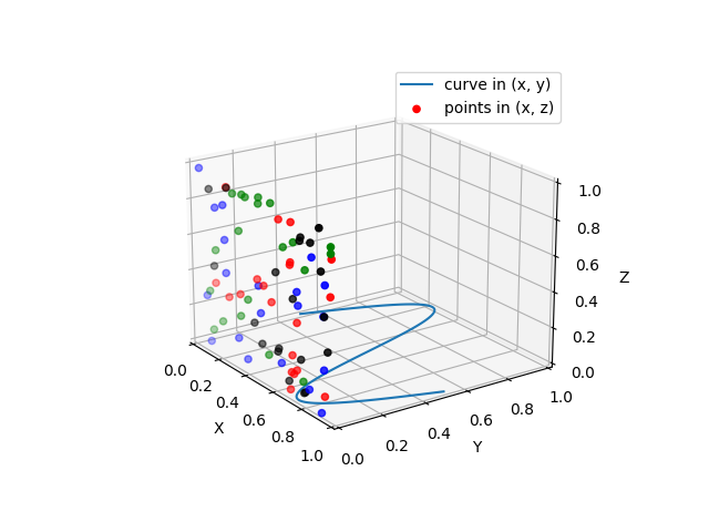
Text#
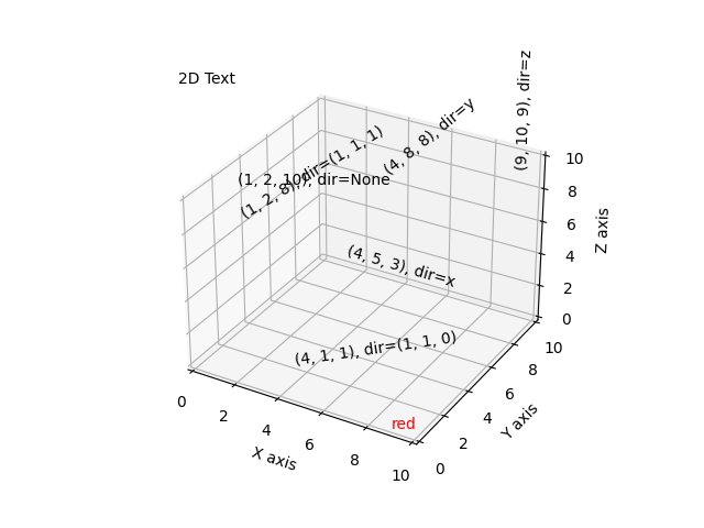
- Axes3D.text(x, y, z, s, zdir=None, **kwargs)[source]#
Add text to the plot. kwargs will be passed on to Axes.text, except for the zdir keyword, which sets the direction to be used as the z direction.
Keywords: matplotlib code example, codex, python plot, pyplot Gallery generated by Sphinx-Gallery