Note
Click here to download the full example code
Contour Demo
Illustrate simple contour plotting, contours on an image with a colorbar for the contours, and labelled contours.
See also the contour image example.
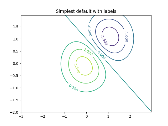
Create a simple contour plot with labels using default colors. The inline argument to clabel will control whether the labels are draw over the line segments of the contour, removing the lines beneath the label
fig, ax = plt.subplots()
CS = ax.contour(X, Y, Z)
ax.clabel(CS, inline=1, fontsize=10)
ax.set_title('Simplest default with labels')
Out:
Text(0.5, 1.0, 'Simplest default with labels')
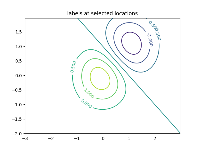
contour labels can be placed manually by providing list of positions (in data coordinate). See ginput_manual_clabel.py for interactive placement.
fig, ax = plt.subplots()
CS = ax.contour(X, Y, Z)
manual_locations = [(-1, -1.4), (-0.62, -0.7), (-2, 0.5), (1.7, 1.2), (2.0, 1.4), (2.4, 1.7)]
ax.clabel(CS, inline=1, fontsize=10, manual=manual_locations)
ax.set_title('labels at selected locations')
Out:
Text(0.5, 1.0, 'labels at selected locations')
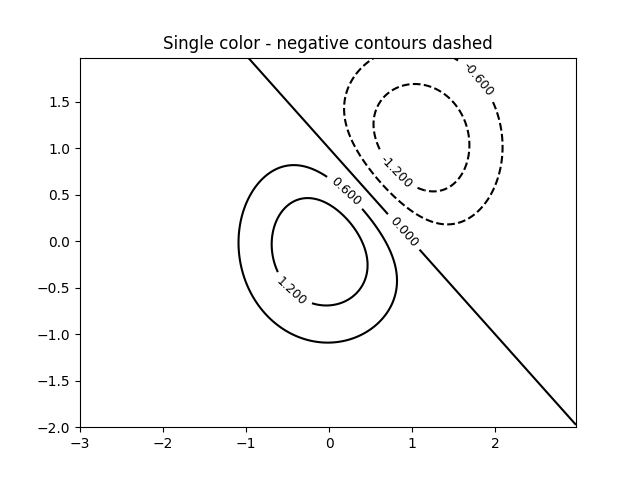
You can force all the contours to be the same color.
fig, ax = plt.subplots()
CS = ax.contour(X, Y, Z, 6, colors='k')  # Negative contours default to dashed.
ax.clabel(CS, fontsize=9, inline=1)
ax.set_title('Single color - negative contours dashed')
Out:
Text(0.5, 1.0, 'Single color - negative contours dashed')
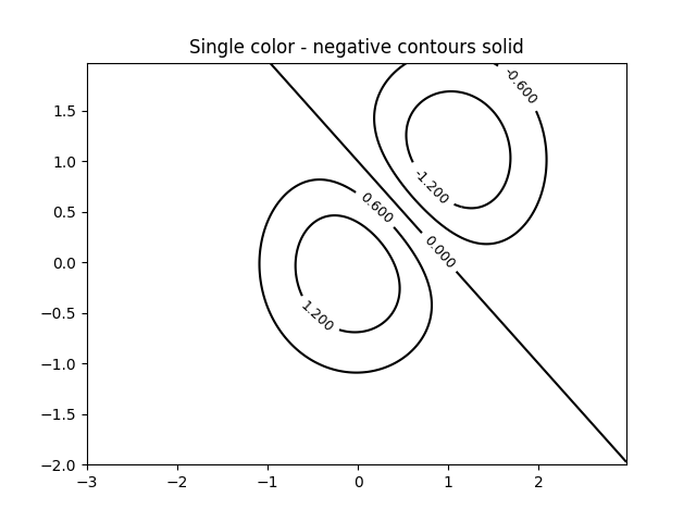
You can set negative contours to be solid instead of dashed:
matplotlib.rcParams['contour.negative_linestyle'] = 'solid'
fig, ax = plt.subplots()
CS = ax.contour(X, Y, Z, 6, colors='k')  # Negative contours default to dashed.
ax.clabel(CS, fontsize=9, inline=1)
ax.set_title('Single color - negative contours solid')
Out:
Text(0.5, 1.0, 'Single color - negative contours solid')
And you can manually specify the colors of the contour
fig, ax = plt.subplots()
CS = ax.contour(X, Y, Z, 6,
                linewidths=np.arange(.5, 4, .5),
                colors=('r', 'green', 'blue', (1, 1, 0), '#afeeee', '0.5'),
                )
ax.clabel(CS, fontsize=9, inline=1)
ax.set_title('Crazy lines')
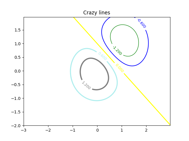
Out:
Text(0.5, 1.0, 'Crazy lines')
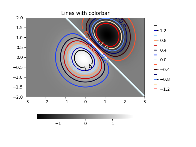
Or you can use a colormap to specify the colors; the default colormap will be used for the contour lines
fig, ax = plt.subplots()
im = ax.imshow(Z, interpolation='bilinear', origin='lower',
                cmap=cm.gray, extent=(-3, 3, -2, 2))
levels = np.arange(-1.2, 1.6, 0.2)
CS = ax.contour(Z, levels, origin='lower', cmap='flag',
                linewidths=2, extent=(-3, 3, -2, 2))

# Thicken the zero contour.
zc = CS.collections[6]
plt.setp(zc, linewidth=4)

ax.clabel(CS, levels[1::2],  # label every second level
          inline=1, fmt='%1.1f', fontsize=14)

# make a colorbar for the contour lines
CB = fig.colorbar(CS, shrink=0.8, extend='both')

ax.set_title('Lines with colorbar')

# We can still add a colorbar for the image, too.
CBI = fig.colorbar(im, orientation='horizontal', shrink=0.8)

# This makes the original colorbar look a bit out of place,
# so let's improve its position.

l, b, w, h = ax.get_position().bounds
ll, bb, ww, hh = CB.ax.get_position().bounds
CB.ax.set_position([ll, b + 0.1*h, ww, h*0.8])

plt.show()
References
The use of the following functions and methods is shown in this example:
Out:
<function _AxesBase.get_position at 0x7fdbd5781790>
Keywords: matplotlib code example, codex, python plot, pyplot Gallery generated by Sphinx-Gallery