Contourf Demo

How to use the axes.Axes.contourf() method to create filled contour plots.

import numpy as np
import matplotlib.pyplot as plt

origin = 'lower'

delta = 0.025

x = y = np.arange(-3.0, 3.01, delta)
X, Y = np.meshgrid(x, y)
Z1 = np.exp(-X**2 - Y**2)
Z2 = np.exp(-(X - 1)**2 - (Y - 1)**2)
Z = (Z1 - Z2) * 2

nr, nc = Z.shape

# put NaNs in one corner:
Z[-nr // 6:, -nc // 6:] = np.nan
# contourf will convert these to masked


Z = np.ma.array(Z)
# mask another corner:
Z[:nr // 6, :nc // 6] = np.ma.masked

# mask a circle in the middle:
interior = np.sqrt(X**2 + Y**2) < 0.5
Z[interior] = np.ma.masked

# We are using automatic selection of contour levels;
# this is usually not such a good idea, because they don't
# occur on nice boundaries, but we do it here for purposes
# of illustration.

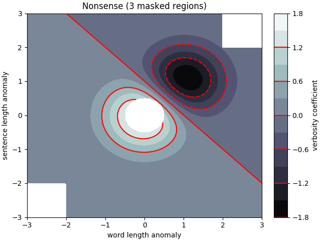
fig1, ax2 = plt.subplots(constrained_layout=True)
CS = ax2.contourf(X, Y, Z, 10, cmap=plt.cm.bone, origin=origin)

# Note that in the following, we explicitly pass in a subset of
# the contour levels used for the filled contours.  Alternatively,
# We could pass in additional levels to provide extra resolution,
# or leave out the levels kwarg to use all of the original levels.

CS2 = ax2.contour(CS, levels=CS.levels[::2], colors='r', origin=origin)

ax2.set_title('Nonsense (3 masked regions)')
ax2.set_xlabel('word length anomaly')
ax2.set_ylabel('sentence length anomaly')

# Make a colorbar for the ContourSet returned by the contourf call.
cbar = fig1.colorbar(CS)
cbar.ax.set_ylabel('verbosity coefficient')
# Add the contour line levels to the colorbar
cbar.add_lines(CS2)

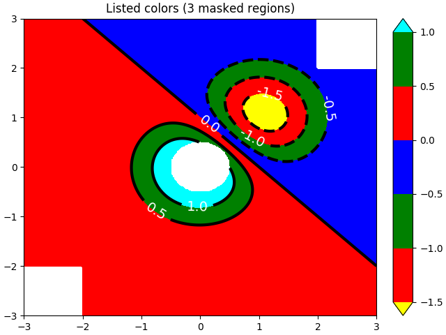
fig2, ax2 = plt.subplots(constrained_layout=True)
# Now make a contour plot with the levels specified,
# and with the colormap generated automatically from a list
# of colors.
levels = [-1.5, -1, -0.5, 0, 0.5, 1]
CS3 = ax2.contourf(X, Y, Z, levels,
                   colors=('r', 'g', 'b'),
                   origin=origin,
                   extend='both')
# Our data range extends outside the range of levels; make
# data below the lowest contour level yellow, and above the
# highest level cyan:
CS3.cmap.set_under('yellow')
CS3.cmap.set_over('cyan')

CS4 = ax2.contour(X, Y, Z, levels,
                  colors=('k',),
                  linewidths=(3,),
                  origin=origin)
ax2.set_title('Listed colors (3 masked regions)')
ax2.clabel(CS4, fmt='%2.1f', colors='w', fontsize=14)

# Notice that the colorbar command gets all the information it
# needs from the ContourSet object, CS3.
fig2.colorbar(CS3)

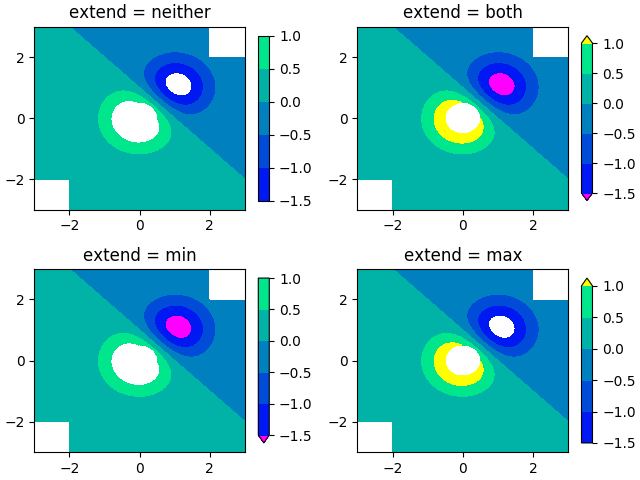
# Illustrate all 4 possible "extend" settings:
extends = ["neither", "both", "min", "max"]
cmap = plt.cm.get_cmap("winter")
cmap.set_under("magenta")
cmap.set_over("yellow")
# Note: contouring simply excludes masked or nan regions, so
# instead of using the "bad" colormap value for them, it draws
# nothing at all in them.  Therefore the following would have
# no effect:
# cmap.set_bad("red")

fig, axs = plt.subplots(2, 2, constrained_layout=True)

for ax, extend in zip(axs.ravel(), extends):
    cs = ax.contourf(X, Y, Z, levels, cmap=cmap, extend=extend, origin=origin)
    fig.colorbar(cs, ax=ax, shrink=0.9)
    ax.set_title("extend = %s" % extend)
    ax.locator_params(nbins=4)

plt.show()

• 
• 
• 

---

References

The use of the following functions, methods and classes is shown in this example:

import matplotlib
matplotlib.axes.Axes.contour
matplotlib.pyplot.contour
matplotlib.axes.Axes.contourf
matplotlib.pyplot.contourf
matplotlib.axes.Axes.clabel
matplotlib.pyplot.clabel
matplotlib.figure.Figure.colorbar
matplotlib.pyplot.colorbar
matplotlib.colors.Colormap
matplotlib.colors.Colormap.set_bad
matplotlib.colors.Colormap.set_under
matplotlib.colors.Colormap.set_over

Out:

<function Colormap.set_over at 0x7fb11f943c80>