Version 3.1.0
Note
Click here to download the full example code
Annotating text with Matplotlib.
The uses of the basic text() will place text
at an arbitrary position on the Axes. A common use case of text is to
annotate some feature of the plot, and the
annotate() method provides helper functionality
to make annotations easy. In an annotation, there are two points to
consider: the location being annotated represented by the argument
xy and the location of the text xytext. Both of these
arguments are (x,y) tuples.
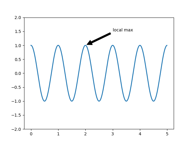
Annotation Basic
In this example, both the xy (arrow tip) and xytext locations
(text location) are in data coordinates. There are a variety of other
coordinate systems one can choose -- you can specify the coordinate
system of xy and xytext with one of the following strings for
xycoords and textcoords (default is 'data')
| argument | coordinate system |
|---|---|
| 'figure points' | points from the lower left corner of the figure |
| 'figure pixels' | pixels from the lower left corner of the figure |
| 'figure fraction' | 0,0 is lower left of figure and 1,1 is upper right |
| 'axes points' | points from lower left corner of axes |
| 'axes pixels' | pixels from lower left corner of axes |
| 'axes fraction' | 0,0 is lower left of axes and 1,1 is upper right |
| 'data' | use the axes data coordinate system |
For example to place the text coordinates in fractional axes coordinates, one could do:
ax.annotate('local max', xy=(3, 1),  xycoords='data',
            xytext=(0.8, 0.95), textcoords='axes fraction',
            arrowprops=dict(facecolor='black', shrink=0.05),
            horizontalalignment='right', verticalalignment='top',
            )
For physical coordinate systems (points or pixels) the origin is the bottom-left of the figure or axes.
Optionally, you can enable drawing of an arrow from the text to the annotated
point by giving a dictionary of arrow properties in the optional keyword
argument arrowprops.
arrowprops key |
description |
|---|---|
| width | the width of the arrow in points |
| frac | the fraction of the arrow length occupied by the head |
| headwidth | the width of the base of the arrow head in points |
| shrink | move the tip and base some percent away from the annotated point and text |
| **kwargs | any key for matplotlib.patches.Polygon,
e.g., facecolor |
In the example below, the xy point is in native coordinates
(xycoords defaults to 'data'). For a polar axes, this is in
(theta, radius) space. The text in this example is placed in the
fractional figure coordinate system. matplotlib.text.Text
keyword args like horizontalalignment, verticalalignment and
fontsize are passed from annotate to the
Text instance.
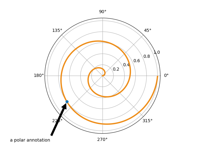
Annotation Polar
For more on all the wild and wonderful things you can do with annotations, including fancy arrows, see Advanced Annotation and Annotating Plots.
Do not proceed unless you have already read Basic annotation,
text() and annotate()!
Let's start with a simple example.
Annotate Text Arrow
The text() function in the pyplot module (or
text method of the Axes class) takes bbox keyword argument, and when
given, a box around the text is drawn.
bbox_props = dict(boxstyle="rarrow,pad=0.3", fc="cyan", ec="b", lw=2)
t = ax.text(0, 0, "Direction", ha="center", va="center", rotation=45,
            size=15,
            bbox=bbox_props)
The patch object associated with the text can be accessed by:
bb = t.get_bbox_patch()
The return value is an instance of FancyBboxPatch and the patch properties like facecolor, edgewidth, etc. can be accessed and modified as usual. To change the shape of the box, use the set_boxstyle method.
bb.set_boxstyle("rarrow", pad=0.6)
The arguments are the name of the box style with its attributes as keyword arguments. Currently, following box styles are implemented.
Class Name Attrs Circle circlepad=0.3 DArrow darrowpad=0.3 LArrow larrowpad=0.3 RArrow rarrowpad=0.3 Round roundpad=0.3,rounding_size=None Round4 round4pad=0.3,rounding_size=None Roundtooth roundtoothpad=0.3,tooth_size=None Sawtooth sawtoothpad=0.3,tooth_size=None Square squarepad=0.3
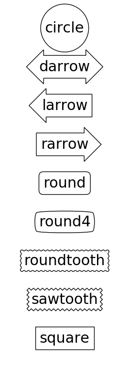
Fancybox Demo
Note that the attribute arguments can be specified within the style name with separating comma (this form can be used as "boxstyle" value of bbox argument when initializing the text instance)
bb.set_boxstyle("rarrow,pad=0.6")
The annotate() function in the pyplot module
(or annotate method of the Axes class) is used to draw an arrow
connecting two points on the plot.
ax.annotate("Annotation",
            xy=(x1, y1), xycoords='data',
            xytext=(x2, y2), textcoords='offset points',
            )
This annotates a point at xy in the given coordinate (xycoords)
with the text at xytext given in textcoords. Often, the
annotated point is specified in the data coordinate and the annotating
text in offset points.
See annotate() for available coordinate systems.
An arrow connecting two points (xy & xytext) can be optionally drawn by
specifying the arrowprops argument. To draw only an arrow, use
empty string as the first argument.
ax.annotate("",
            xy=(0.2, 0.2), xycoords='data',
            xytext=(0.8, 0.8), textcoords='data',
            arrowprops=dict(arrowstyle="->",
                            connectionstyle="arc3"),
            )
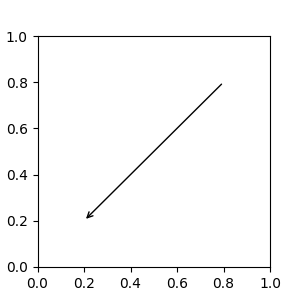
Annotate Simple01
The arrow drawing takes a few steps.
connectionstyle key value.arrowstyle key value.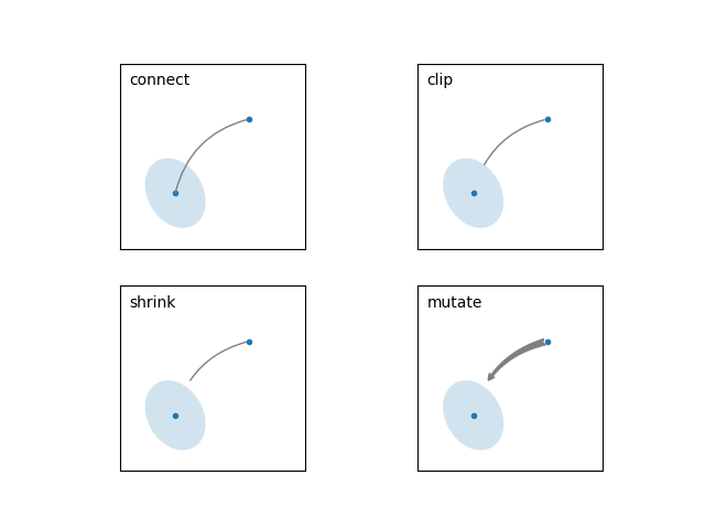
Annotate Explain
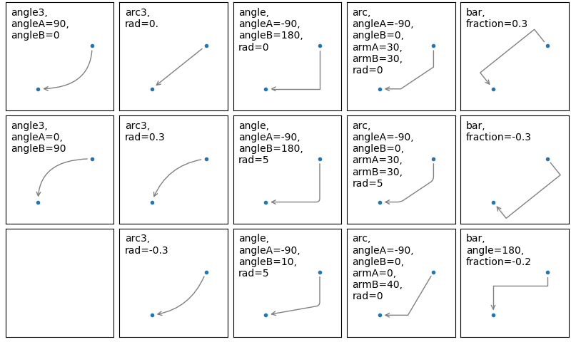
The creation of the connecting path between two points is controlled by
connectionstyle key and the following styles are available.
Name Attrs angleangleA=90,angleB=0,rad=0.0 angle3angleA=90,angleB=0 arcangleA=0,angleB=0,armA=None,armB=None,rad=0.0 arc3rad=0.0 bararmA=0.0,armB=0.0,fraction=0.3,angle=None
Note that "3" in angle3 and arc3 is meant to indicate that the
resulting path is a quadratic spline segment (three control
points). As will be discussed below, some arrow style options can only
be used when the connecting path is a quadratic spline.
The behavior of each connection style is (limitedly) demonstrated in the
example below. (Warning : The behavior of the bar style is currently not
well defined, it may be changed in the future).
Connectionstyle Demo
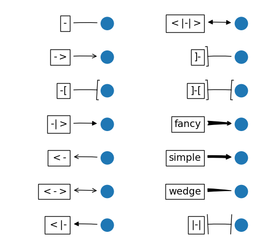
The connecting path (after clipping and shrinking) is then mutated to
an arrow patch, according to the given arrowstyle.
Name Attrs -None ->head_length=0.4,head_width=0.2 -[widthB=1.0,lengthB=0.2,angleB=None |-|widthA=1.0,widthB=1.0 -|>head_length=0.4,head_width=0.2 <-head_length=0.4,head_width=0.2 <->head_length=0.4,head_width=0.2 <|-head_length=0.4,head_width=0.2 <|-|>head_length=0.4,head_width=0.2 fancyhead_length=0.4,head_width=0.4,tail_width=0.4 simplehead_length=0.5,head_width=0.5,tail_width=0.2 wedgetail_width=0.3,shrink_factor=0.5
Fancyarrow Demo
Some arrowstyles only work with connection styles that generate a
quadratic-spline segment. They are fancy, simple, and wedge.
For these arrow styles, you must use the "angle3" or "arc3" connection
style.
If the annotation string is given, the patchA is set to the bbox patch of the text by default.
Annotate Simple02
As in the text command, a box around the text can be drawn using
the bbox argument.
Annotate Simple03
By default, the starting point is set to the center of the text
extent. This can be adjusted with relpos key value. The values
are normalized to the extent of the text. For example, (0,0) means
lower-left corner and (1,1) means top-right.
Annotate Simple04
There are classes of artists that can be placed at an anchored location
in the Axes. A common example is the legend. This type of artist can
be created by using the OffsetBox class. A few predefined classes are
available in mpl_toolkits.axes_grid1.anchored_artists others in
matplotlib.offsetbox
from matplotlib.offsetbox import AnchoredText
at = AnchoredText("Figure 1a",
                  prop=dict(size=15), frameon=True,
                  loc='upper left',
                  )
at.patch.set_boxstyle("round,pad=0.,rounding_size=0.2")
ax.add_artist(at)
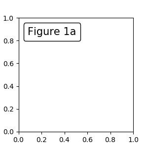
Anchored Box01
The loc keyword has same meaning as in the legend command.
A simple application is when the size of the artist (or collection of
artists) is known in pixel size during the time of creation. For
example, If you want to draw a circle with fixed size of 20 pixel x 20
pixel (radius = 10 pixel), you can utilize
AnchoredDrawingArea. The instance is created with a size of the
drawing area (in pixels), and arbitrary artists can added to the
drawing area. Note that the extents of the artists that are added to
the drawing area are not related to the placement of the drawing
area itself. Only the initial size matters.
from mpl_toolkits.axes_grid1.anchored_artists import AnchoredDrawingArea

ada = AnchoredDrawingArea(20, 20, 0, 0,
                          loc='upper right', pad=0., frameon=False)
p1 = Circle((10, 10), 10)
ada.drawing_area.add_artist(p1)
p2 = Circle((30, 10), 5, fc="r")
ada.drawing_area.add_artist(p2)
The artists that are added to the drawing area should not have a transform set (it will be overridden) and the dimensions of those artists are interpreted as a pixel coordinate, i.e., the radius of the circles in above example are 10 pixels and 5 pixels, respectively.
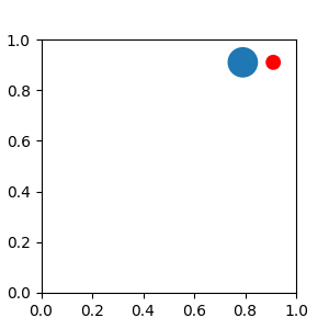
Anchored Box02
Sometimes, you want your artists to scale with the data coordinate (or
coordinates other than canvas pixels). You can use
AnchoredAuxTransformBox class. This is similar to
AnchoredDrawingArea except that the extent of the artist is
determined during the drawing time respecting the specified transform.
from mpl_toolkits.axes_grid1.anchored_artists import AnchoredAuxTransformBox

box = AnchoredAuxTransformBox(ax.transData, loc='upper left')
el = Ellipse((0,0), width=0.1, height=0.4, angle=30)  # in data coordinates!
box.drawing_area.add_artist(el)
The ellipse in the above example will have width and height corresponding to 0.1 and 0.4 in data coordinates and will be automatically scaled when the view limits of the axes change.
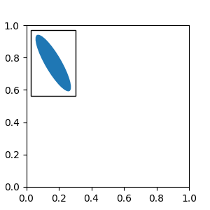
Anchored Box03
As in the legend, the bbox_to_anchor argument can be set. Using the HPacker and VPacker, you can have an arrangement(?) of artist as in the legend (as a matter of fact, this is how the legend is created).
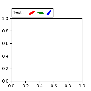
Anchored Box04
Note that unlike the legend, the bbox_transform is set
to IdentityTransform by default.
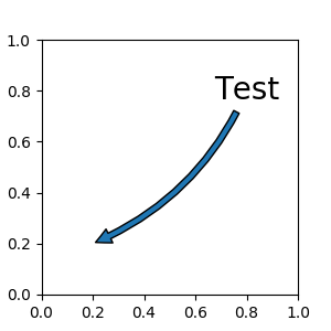
The Annotation in matplotlib supports several types of coordinates as described in Basic annotation. For an advanced user who wants more control, it supports a few other options.
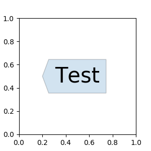
Transforminstance. For example,ax.annotate("Test", xy=(0.5, 0.5), xycoords=ax.transAxes)is identical to
ax.annotate("Test", xy=(0.5, 0.5), xycoords="axes fraction")With this, you can annotate a point in other axes.
ax1, ax2 = subplot(121), subplot(122)
ax2.annotate("Test", xy=(0.5, 0.5), xycoords=ax1.transData,
             xytext=(0.5, 0.5), textcoords=ax2.transData,
             arrowprops=dict(arrowstyle="->"))
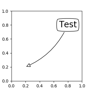
Artistinstance. The xy value (or xytext) is interpreted as a fractional coordinate of the bbox (return value of get_window_extent) of the artist.an1 = ax.annotate("Test 1", xy=(0.5, 0.5), xycoords="data", va="center", ha="center", bbox=dict(boxstyle="round", fc="w")) an2 = ax.annotate("Test 2", xy=(1, 0.5), xycoords=an1, # (1,0.5) of the an1's bbox xytext=(30,0), textcoords="offset points", va="center", ha="left", bbox=dict(boxstyle="round", fc="w"), arrowprops=dict(arrowstyle="->"))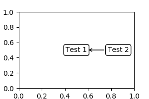
Annotation with Simple Coordinates
Note that it is your responsibility that the extent of the coordinate artist (an1 in above example) is determined before an2 gets drawn. In most cases, it means that an2 needs to be drawn later than an1.
A callable object that returns an instance of either
BboxBaseorTransform. If a transform is returned, it is the same as 1 and if a bbox is returned, it is the same as 2. The callable object should take a single argument of the renderer instance. For example, the following two commands give identical resultsan2 = ax.annotate("Test 2", xy=(1, 0.5), xycoords=an1, xytext=(30,0), textcoords="offset points") an2 = ax.annotate("Test 2", xy=(1, 0.5), xycoords=an1.get_window_extent, xytext=(30,0), textcoords="offset points")A tuple of two coordinate specifications. The first item is for the x-coordinate and the second is for the y-coordinate. For example,
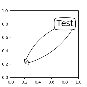
annotate("Test", xy=(0.5, 1), xycoords=("data", "axes fraction"))0.5 is in data coordinates, and 1 is in normalized axes coordinates. You may use an artist or transform as with a tuple. For example,
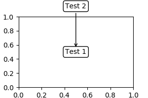
Annotation with Simple Coordinates 2
Sometimes, you want your annotation with some "offset points", not from the annotated point but from some other point.
OffsetFromis a helper class for such cases.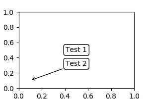
Annotation with Simple Coordinates 3
You may take a look at this example Annotating Plots.
The ConnectionPatch is like an annotation without text. While the annotate function is recommended in most situations, the ConnectionPatch is useful when you want to connect points in different axes.
from matplotlib.patches import ConnectionPatch
xy = (0.2, 0.2)
con = ConnectionPatch(xyA=xy, xyB=xy, coordsA="data", coordsB="data",
                      axesA=ax1, axesB=ax2)
ax2.add_artist(con)
The above code connects point xy in the data coordinates of ax1 to
point xy in the data coordinates of ax2. Here is a simple example.
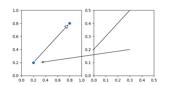
Connect Simple01
While the ConnectionPatch instance can be added to any axes, you may want to add it to the axes that is latest in drawing order to prevent overlap by other axes.
mpl_toolkits.axes_grid1.inset_locator defines some patch classes useful
for interconnecting two axes. Understanding the code requires some
knowledge of how mpl's transform works. But, utilizing it will be
straight forward.
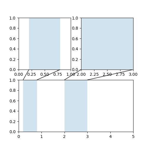
Axes Zoom Effect
You can use a custom box style. The value for the boxstyle can be a
callable object in the following forms.:
def __call__(self, x0, y0, width, height, mutation_size,
             aspect_ratio=1.):
    '''
    Given the location and size of the box, return the path of
    the box around it.

      - *x0*, *y0*, *width*, *height* : location and size of the box
      - *mutation_size* : a reference scale for the mutation.
      - *aspect_ratio* : aspect-ratio for the mutation.
    '''
    path = ...
    return path
Here is a complete example.
Custom Boxstyle01
However, it is recommended that you derive from the matplotlib.patches.BoxStyle._Base as demonstrated below.
Custom Boxstyle02
Similarly, you can define a custom ConnectionStyle and a custom ArrowStyle.
See the source code of lib/matplotlib/patches.py and check
how each style class is defined.
Keywords: matplotlib code example, codex, python plot, pyplot Gallery generated by Sphinx-Gallery