Version 3.0.2
The examples have been migrated to use sphinx gallery. This allows better mixing of prose and code in the examples, provides links to download the examples as both a Python script and a Jupyter notebook, and improves the thumbnail galleries. The examples have been re-organized into Tutorials and a Gallery.
Many docstrings and examples have been clarified and improved.
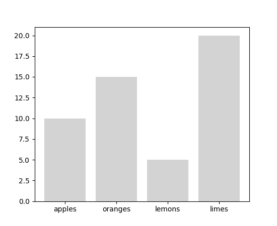
All plotting functions now support string categorical values as input. For example:
data = {'apples': 10, 'oranges': 15, 'lemons': 5, 'limes': 20}
fig, ax = plt.subplots()
ax.bar(data.keys(), data.values(), color='lightgray')
(Source code, png, pdf)

Jake Vanderplas' JSAnimation package has been merged into Matplotlib. This
adds to Matplotlib the HTMLWriter class for
generating a JavaScript HTML animation, suitable for the IPython notebook.
This can be activated by default by setting the animation.html rc
parameter to jshtml. One can also call the
to_jshtml method to manually convert an
animation. This can be displayed using IPython's HTML display class:
from IPython.display import HTML
HTML(animation.to_jshtml())
The HTMLWriter class can also be used to generate
an HTML file by asking for the html writer.
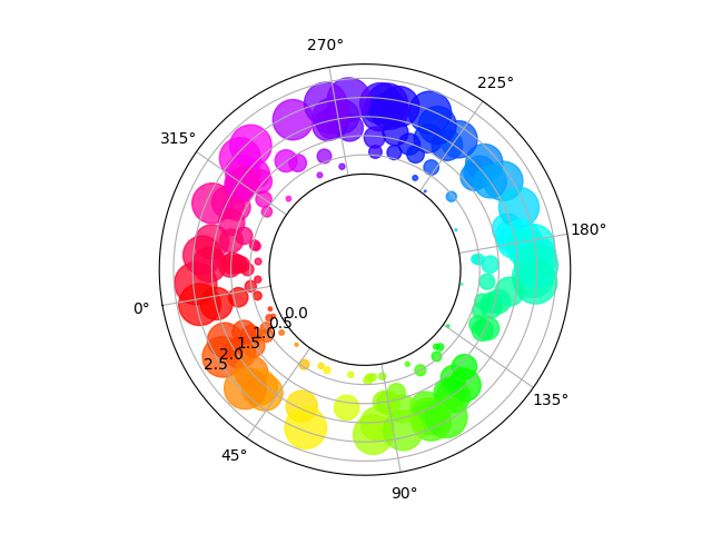
The polar axes transforms have been greatly re-factored to allow for more customization of view limits and tick labelling. Additional options for view limits allow for creating an annulus, a sector, or some combination of the two.
The set_rorigin() method may
be used to provide an offset to the minimum plotting radius, producing an
annulus.
The set_theta_zero_location()
method now has an optional offset argument. This argument may be used
to further specify the zero location based on the given anchor point.
Polar Offset Demo
The set_thetamin() and
set_thetamax() methods may
be used to limit the range of angles plotted, producing sectors of a circle.
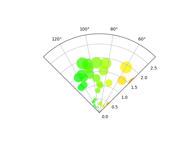
Polar Sector Demo
Previous releases allowed plots containing negative radii for which the negative values are simply used as labels, and the real radius is shifted by the configured minimum. This release also allows negative radii to be used for grids and ticks, which were previously silently ignored.
Radial ticks have been modified to be parallel to the circular grid line, and
angular ticks have been modified to be parallel to the grid line. It may also
be useful to rotate tick labels to match the boundary. Calling
ax.tick_params(rotation='auto') will enable the new behavior: radial tick
labels will be parallel to the circular grid line, and angular tick labels will
be perpendicular to the grid line (i.e., parallel to the outer boundary).
Additionally, tick labels now obey the padding settings that previously only
worked on Cartesian plots. Consequently, the frac argument to
PolarAxes.set_thetagrids is no longer applied. Tick padding can be modified
with the pad argument to Axes.tick_params or Axis.set_tick_params.
Figure class now has subplots method¶The Figure class now has a
subplots() method which behaves the same as
pyplot.subplots() but on an existing figure.
savefig() now accepts metadata as a keyword
argument. It can be used to store key/value pairs in the image metadata.
writeInfoDict() for a list of
supported keywords)plt.savefig('test.png', metadata={'Software': 'My awesome software'})
The interactive GUI backends will now change the cursor to busy when Matplotlib is rendering the canvas.
A PolygonSelector class has been added to
matplotlib.widgets. See
Polygon Selector Demo for details.
matplotlib.ticker.PercentFormatter¶The new PercentFormatter formatter has some nice
features like being able to convert from arbitrary data scales to
percents, a customizable percent symbol and either automatic or manual
control over the decimal points.
The SOURCE_DATE_EPOCH environment variable can now be used to set
the timestamp value in the PS and PDF outputs. See source date epoch.
Alternatively, calling savefig with metadata={'CreationDate': None}
will omit the timestamp altogether for the PDF backend.
The reproducibility of the output from the PS and PDF backends has so
far been tested using various plot elements but only default values of
options such as {ps,pdf}.fonttype that can affect the output at a
low level, and not with the mathtext or usetex features. When
Matplotlib calls external tools (such as PS distillers or LaTeX) their
versions need to be kept constant for reproducibility, and they may
add sources of nondeterminism outside the control of Matplotlib.
For SVG output, the svg.hashsalt rc parameter has been added in an
earlier release. This parameter changes some random identifiers in the
SVG file to be deterministic. The downside of this setting is that if
more than one file is generated using deterministic identifiers
and they end up as parts of one larger document, the identifiers can
collide and cause the different parts to affect each other.
These features are now enabled in the tests for the PDF and SVG backends, so most test output files (but not all of them) are now deterministic.
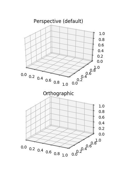
Axes3D now accepts proj_type keyword
argument and has a method set_proj_type().
The default option is 'persp' as before, and supplying 'ortho' enables
orthographic view.
Compare the z-axis which is vertical in orthographic view, but slightly skewed in the perspective view.
import numpy as np
import matplotlib.pyplot as plt
from mpl_toolkits.mplot3d import Axes3D

fig = plt.figure(figsize=(4, 6))
ax1 = fig.add_subplot(2, 1, 1, projection='3d')
ax1.set_proj_type('persp')
ax1.set_title('Perspective (default)')

ax2 = fig.add_subplot(2, 1, 2, projection='3d')
ax2.set_proj_type('ortho')
ax2.set_title('Orthographic')

plt.show()
(Source code, png, pdf)
get_status function¶A get_status() method has been added to
the matplotlib.widgets.CheckButtons class. This get_status method
allows user to query the status (True/False) of all of the buttons in the
CheckButtons object.
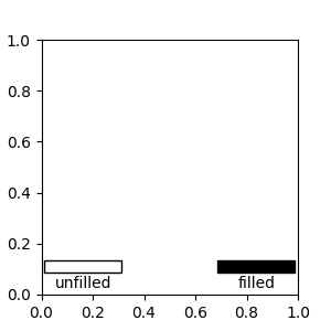
fill_bar argument to AnchoredSizeBar¶The mpl_toolkits class
AnchoredSizeBar now has an
additional fill_bar argument, which makes the size bar a solid rectangle
instead of just drawing the border of the rectangle. The default is None,
and whether or not the bar will be filled by default depends on the value of
size_vertical. If size_vertical is nonzero, fill_bar will be set to
True. If size_vertical is zero then fill_bar will be set to
False. If you wish to override this default behavior, set fill_bar to
True or False to unconditionally always or never use a filled patch
rectangle for the size bar.
import matplotlib.pyplot as plt
from mpl_toolkits.axes_grid1.anchored_artists import AnchoredSizeBar

fig, ax = plt.subplots(figsize=(3, 3))

bar0 = AnchoredSizeBar(ax.transData, 0.3, 'unfilled', loc='lower left',
                       frameon=False, size_vertical=0.05, fill_bar=False)
ax.add_artist(bar0)
bar1 = AnchoredSizeBar(ax.transData, 0.3, 'filled', loc='lower right',
                       frameon=False, size_vertical=0.05, fill_bar=True)
ax.add_artist(bar1)

plt.show()
(Source code, png, pdf)

Annotations now use the default arrow style when setting arrowprops={},
rather than no arrow (the new behavior actually matches the documentation).
When using the quiver() and
barbs() plotting methods, it is now possible to
pass dates, just like for other methods like plot().
This also allows these functions to handle values that need unit-conversion
applied.
The default linecolor keyword argument for hexbin()
is now 'face', and supplying 'none' now prevents lines from being drawn
around the hexagons.
Calling Figure.legend() can now be done with no arguments. In this case
a legend will be created that contains all the artists on all the axes
contained within the figure.
A legend entry can now contain more than one legend key. The extended
HandlerTuple class now accepts two parameters:
ndivide divides the legend area in the specified number of sections;
pad changes the padding between the legend keys.
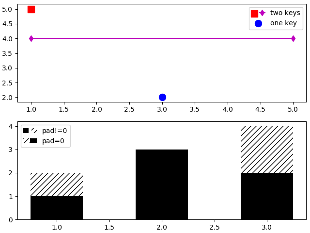
Multiple Legend Keys
clear for figure()¶When the pyplot's function figure() is called
with a num parameter, a new window is only created if no existing
window with the same value exists. A new bool parameter clear was
added for explicitly clearing its existing contents. This is particularly
useful when utilized in interactive sessions. Since
subplots() also accepts keyword arguments
from figure(), it can also be used there:
import matplotlib.pyplot as plt

fig0 = plt.figure(num=1)
fig0.suptitle("A fancy plot")
print("fig0.texts: ", [t.get_text() for t in fig0.texts])

fig1 = plt.figure(num=1, clear=False)  # do not clear contents of window
fig1.text(0.5, 0.5, "Really fancy!")
print("fig0 is fig1: ",  fig0 is fig1)
print("fig1.texts: ", [t.get_text() for t in fig1.texts])

fig2, ax2 = plt.subplots(2, 1, num=1, clear=True)  # clear contents
print("fig0 is fig2: ",  fig0 is fig2)
print("fig2.texts: ", [t.get_text() for t in fig2.texts])

# The output:
# fig0.texts:  ['A fancy plot']
# fig0 is fig1:  True
# fig1.texts:  ['A fancy plot', 'Really fancy!']
# fig0 is fig2:  True
# fig2.texts:  []
LogFormatterMathtext¶LogFormatterMathtext now includes the
option to specify a minimum value exponent to format as a scalar
(i.e., 0.001 instead of 10-3).
Plotting a quiverkey() now admits the
angle keyword argument, which sets the angle at which to draw the
key arrow.
The methods matplotlib.colors.LinearSegmentedColormap.reversed() and
matplotlib.colors.ListedColormap.reversed() return a reversed
instance of the Colormap. This implements a way for any Colormap to be
reversed.
Artist.setp (and pyplot.setp) accept a file argument¶The argument is keyword-only. It allows an output file other than
sys.stdout to be specified. It works exactly like the file argument
to print.
streamplot streamline generation more configurable¶The starting point, direction, and length of the stream lines can now be configured. This allows to follow the vector field for a longer time and can enhance the visibility of the flow pattern in some use cases.
Axis.set_tick_params now responds to rotation¶Bulk setting of tick label rotation is now possible via
tick_params() using the rotation
keyword.
ax.tick_params(which='both', rotation=90)
Internally, the Tick's label1On() attribute
is now used to hide tick labels instead of setting the visibility on the tick
label objects.
This improves overall performance and fixes some issues.
As a consequence, in case those labels ought to be shown,
tick_params()
needs to be used, e.g.
ax.tick_params(labelbottom=True)
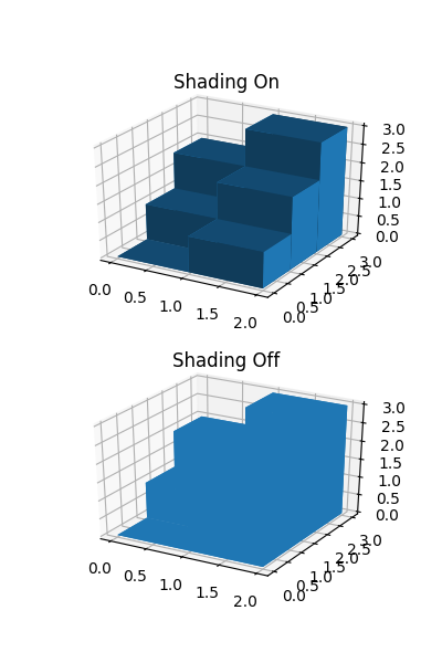
A new shade parameter has been added the 3D
bar plotting method. The default behavior
remains to shade the bars, but now users have the option of setting shade
to False.
import numpy as np
import matplotlib.pyplot as plt
from mpl_toolkits.mplot3d import Axes3D

x = np.arange(2)
y = np.arange(3)
x2d, y2d = np.meshgrid(x, y)
x, y = x2d.ravel(), y2d.ravel()
z = np.zeros_like(x)
dz = x + y

fig = plt.figure(figsize=(4, 6))
ax1 = fig.add_subplot(2, 1, 1, projection='3d')
ax1.bar3d(x, y, z, 1, 1, dz, shade=True)
ax1.set_title('Shading On')

ax2 = fig.add_subplot(2, 1, 2, projection='3d')
ax2.bar3d(x, y, z, 1, 1, dz, shade=False)
ax2.set_title('Shading Off')

plt.show()
(Source code, png, pdf)
which Parameter for autofmt_xdate¶A which parameter now exists for the method
autofmt_xdate(). This allows a user to format
major, minor or both tick labels selectively. The
default behavior will rotate and align the major tick labels.
fig.autofmt_xdate(bottom=0.2, rotation=30, ha='right', which='minor')
subplot2grid¶A fig parameter now exists for the function
subplot2grid(). This allows a user to specify the
figure where the subplots will be created. If fig is None (default)
then the method will use the current figure retrieved by
gcf().
subplot2grid(shape, loc, rowspan=1, colspan=1, fig=myfig)
fill_betweenx¶The interpolate parameter now exists for the method
fill_betweenx(). This allows a user to
interpolate the data and fill the areas in the crossover points,
similarly to fill_between().
sep for EngFormatter¶A new sep keyword argument has been added to
EngFormatter and provides a means to
define the string that will be used between the value and its
unit. The default string is " ", which preserves the former
behavior. Additionally, the separator is now present between the value
and its unit even in the absence of SI prefix. There was formerly a
bug that was causing strings like "3.14V" to be returned instead of
the expected "3.14 V" (with the default behavior).
MATPLOTLIBRC behavior¶The environmental variable can now specify the full file path or the
path to a directory containing a matplotlibrc file.
A newly added TransformedPatchPath provides a
means to transform a Patch into a
Path via a Transform
while caching the resulting path. If neither the patch nor the transform have
changed, a cached copy of the path is returned.
This class differs from the older
TransformedPath in that it is able to refresh
itself based on the underlying patch while the older class uses an immutable
path.
The new AbstractMovieWriter class defines
the API required by a class that is to be used as the writer in the
matplotlib.animation.Animation.save() method. The existing
MovieWriter class now derives from the new
abstract base class.
The validation of rcParams that are related to line styles
(lines.linestyle, boxplot.*.linestyle, grid.linestyle and
contour.negative_linestyle) now effectively checks that the values
are valid line styles. Strings like 'dashed' or '--' are
accepted, as well as even-length sequences of on-off ink like [1,
1.65]. In this latter case, the offset value is handled internally
and should not be provided by the user.
The new validation scheme replaces the former one used for the
contour.negative_linestyle rcParams, that was limited to
'solid' and 'dashed' line styles.
The validation is case-insensitive. The following are now valid:
grid.linestyle             : (1, 3)   # loosely dotted grid lines
contour.negative_linestyle : dashdot  # previously only solid or dashed
The automated tests have been switched from nose to pytest.
Line simplification controlled by the path.simplify and
path.simplify_threshold parameters has been improved. You should
notice better rendering performance when plotting large amounts of
data (as long as the above parameters are set accordingly). Only the
line segment portion of paths will be simplified -- if you are also
drawing markers and experiencing problems with rendering speed, you
should consider using the markevery option to plot.
See the Performance section in the usage tutorial for more
information.
The simplification works by iteratively merging line segments
into a single vector until the next line segment's perpendicular
distance to the vector (measured in display-coordinate space)
is greater than the path.simplify_threshold parameter. Thus, higher
values of path.simplify_threshold result in quicker rendering times.
If you are plotting just to explore data and not for publication quality,
pixel perfect plots, then a value of 1.0 can be safely used. If you
want to make sure your plot reflects your data exactly, then you should
set path.simplify to false and/or path.simplify_threshold to 0.
Matplotlib currently defaults to a conservative value of 1/9, smaller
values are unlikely to cause any visible differences in your plots.
intersects_bbox() has been implemented in
c++ which improves the performance of automatically placing the legend.