

(Source code, png, pdf)
"""This is a ported version of a MATLAB example from the signal
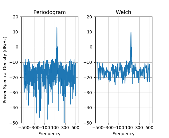
processing toolbox that showed some difference at one time between
Matplotlib's and MATLAB's scaling of the PSD.
This differs from psd_demo3.py in that this uses a complex signal,
so we can see that complex PSD's work properly
"""
import numpy as np
import matplotlib.pyplot as plt
import matplotlib.mlab as mlab
prng = np.random.RandomState(123456) # to ensure reproducibility
fs = 1000
t = np.linspace(0, 0.3, 301)
A = np.array([2, 8]).reshape(-1, 1)
f = np.array([150, 140]).reshape(-1, 1)
xn = (A * np.exp(2j * np.pi * f * t)).sum(axis=0) + 5 * prng.randn(*t.shape)
fig, (ax0, ax1) = plt.subplots(ncols=2)
fig.subplots_adjust(hspace=0.45, wspace=0.3)
yticks = np.arange(-50, 30, 10)
yrange = (yticks[0], yticks[-1])
xticks = np.arange(-500, 550, 200)
ax0.psd(xn, NFFT=301, Fs=fs, window=mlab.window_none, pad_to=1024,
scale_by_freq=True)
ax0.set_title('Periodogram')
ax0.set_yticks(yticks)
ax0.set_xticks(xticks)
ax0.grid(True)
ax0.set_ylim(yrange)
ax1.psd(xn, NFFT=150, Fs=fs, window=mlab.window_none, pad_to=512, noverlap=75,
scale_by_freq=True)
ax1.set_title('Welch')
ax1.set_xticks(xticks)
ax1.set_yticks(yticks)
ax1.set_ylabel('') # overwrite the y-label added by `psd`
ax1.grid(True)
ax1.set_ylim(yrange)
plt.show()
Keywords: python, matplotlib, pylab, example, codex (see Search examples)