Note
Click here to download the full example code
Annotations#
Annotations are graphical elements, often pieces of text, that explain, add
context to, or otherwise highlight some portion of the visualized data.
annotate supports a number of coordinate systems for flexibly
positioning data and annotations relative to each other and a variety of
options of for styling the text. Axes.annotate also provides an optional arrow
from the text to the data and this arrow can be styled in various ways.
text can also be used for simple text annotation, but does not
provide as much flexibility in positioning and styling as annotate.
Basic annotation#
In an annotation, there are two points to consider: the location of the data
being annotated xy and the location of the annotation text xytext. Both
of these arguments are (x, y) tuples:

In this example, both the xy (arrow tip) and xytext locations (text location) are in data coordinates. There are a variety of other coordinate systems one can choose -- you can specify the coordinate system of xy and xytext with one of the following strings for xycoords and textcoords (default is 'data')
argument |
coordinate system |
|---|---|
'figure points' |
points from the lower left corner of the figure |
'figure pixels' |
pixels from the lower left corner of the figure |
'figure fraction' |
(0, 0) is lower left of figure and (1, 1) is upper right |
'axes points' |
points from lower left corner of axes |
'axes pixels' |
pixels from lower left corner of axes |
'axes fraction' |
(0, 0) is lower left of axes and (1, 1) is upper right |
'data' |
use the axes data coordinate system |
The following strings are also valid arguments for textcoords
argument |
coordinate system |
|---|---|
'offset points' |
offset (in points) from the xy value |
'offset pixels' |
offset (in pixels) from the xy value |
For physical coordinate systems (points or pixels) the origin is the bottom-left of the figure or axes. Points are typographic points meaning that they are a physical unit measuring 1/72 of an inch. Points and pixels are discussed in further detail in Plotting in physical coordinates.
Annotating data#
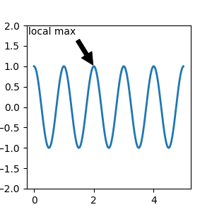
This example places the text coordinates in fractional axes coordinates:
fig, ax = plt.subplots(figsize=(3, 3))

t = np.arange(0.0, 5.0, 0.01)
s = np.cos(2*np.pi*t)
line, = ax.plot(t, s, lw=2)

ax.annotate('local max', xy=(2, 1), xycoords='data',
            xytext=(0.01, .99), textcoords='axes fraction',
            va='top', ha='left',
            arrowprops=dict(facecolor='black', shrink=0.05))
ax.set_ylim(-2, 2)
Annotating with arrows#
You can enable drawing of an arrow from the text to the annotated point by giving a dictionary of arrow properties in the optional keyword argument arrowprops.
arrowprops key |
description |
|---|---|
width |
the width of the arrow in points |
frac |
the fraction of the arrow length occupied by the head |
headwidth |
the width of the base of the arrow head in points |
shrink |
move the tip and base some percent away from the annotated point and text |
**kwargs |
any key for |
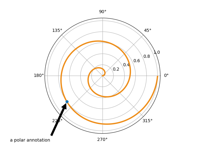
In the example below, the xy point is in the data coordinate system
since xycoords defaults to 'data'. For a polar axes, this is in
(theta, radius) space. The text in this example is placed in the
fractional figure coordinate system. matplotlib.text.Text
keyword arguments like horizontalalignment, verticalalignment and
fontsize are passed from annotate to the
Text instance.
fig = plt.figure()
ax = fig.add_subplot(projection='polar')
r = np.arange(0, 1, 0.001)
theta = 2 * 2*np.pi * r
line, = ax.plot(theta, r, color='#ee8d18', lw=3)

ind = 800
thisr, thistheta = r[ind], theta[ind]
ax.plot([thistheta], [thisr], 'o')
ax.annotate('a polar annotation',
            xy=(thistheta, thisr),  # theta, radius
            xytext=(0.05, 0.05),    # fraction, fraction
            textcoords='figure fraction',
            arrowprops=dict(facecolor='black', shrink=0.05),
            horizontalalignment='left',
            verticalalignment='bottom')
For more on plotting with arrows, see Customizing annotation arrows
Placing text annotations relative to data#
Annotations can be positioned at a relative offset to the xy input to
annotation by setting the textcoords keyword argument to 'offset points'
or 'offset pixels'.
fig, ax = plt.subplots(figsize=(3, 3))
x = [1, 3, 5, 7, 9]
y = [2, 4, 6, 8, 10]
annotations = ["A", "B", "C", "D", "E"]
ax.scatter(x, y, s=20)

for xi, yi, text in zip(x, y, annotations):
    ax.annotate(text,
                xy=(xi, yi), xycoords='data',
                xytext=(1.5, 1.5), textcoords='offset points')
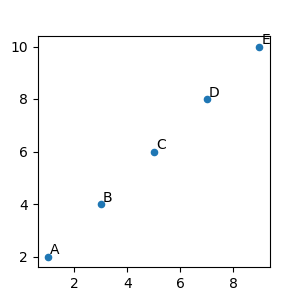
The annotations are offset 1.5 points (1.5*1/72 inches) from the xy values.
Advanced annotation#
We recommend reading Basic annotation, text()
and annotate() before reading this section.
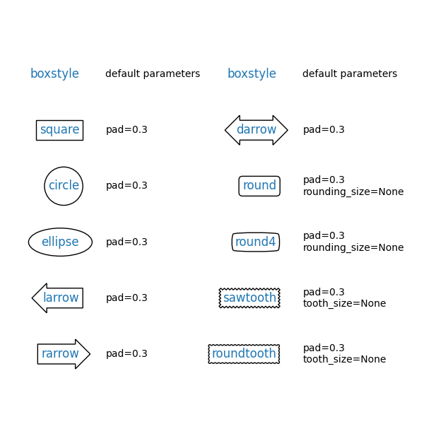
Annotating with boxed text#
text takes a bbox keyword argument, which draws a box around the
text:
fig, ax = plt.subplots(figsize=(5, 5))
t = ax.text(0.5, 0.5, "Direction",
            ha="center", va="center", rotation=45, size=15,
            bbox=dict(boxstyle="rarrow,pad=0.3",
                      fc="lightblue", ec="steelblue", lw=2))
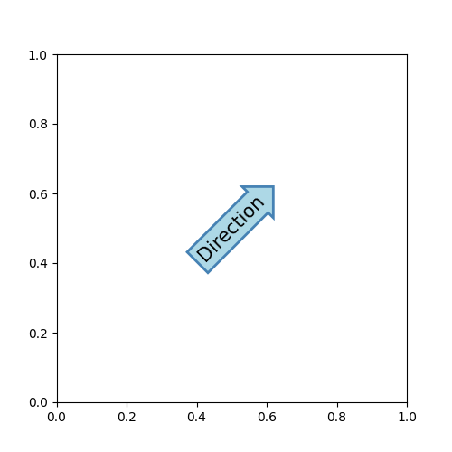
The arguments are the name of the box style with its attributes as keyword arguments. Currently, following box styles are implemented.
Class
Name
Attrs
Circle
circlepad=0.3
DArrow
darrowpad=0.3
Ellipse
ellipsepad=0.3
LArrow
larrowpad=0.3
RArrow
rarrowpad=0.3
Round
roundpad=0.3,rounding_size=None
Round4
round4pad=0.3,rounding_size=None
Roundtooth
roundtoothpad=0.3,tooth_size=None
Sawtooth
sawtoothpad=0.3,tooth_size=None
Square
squarepad=0.3
The patch object (box) associated with the text can be accessed using:
bb = t.get_bbox_patch()
The return value is a FancyBboxPatch; patch properties
(facecolor, edgewidth, etc.) can be accessed and modified as usual.
FancyBboxPatch.set_boxstyle sets the box shape:
bb.set_boxstyle("rarrow", pad=0.6)
The attribute arguments can also be specified within the style name with separating comma:
bb.set_boxstyle("rarrow, pad=0.6")
Defining custom box styles#
You can use a custom box style. The value for the boxstyle can be a
callable object in the following forms:
from matplotlib.path import Path


def custom_box_style(x0, y0, width, height, mutation_size):
    """
    Given the location and size of the box, return the path of the box around
    it. Rotation is automatically taken care of.

    Parameters
    ----------
    x0, y0, width, height : float
       Box location and size.
    mutation_size : float
    Mutation reference scale, typically the text font size.
    """
    # padding
    mypad = 0.3
    pad = mutation_size * mypad
    # width and height with padding added.
    width = width + 2 * pad
    height = height + 2 * pad
    # boundary of the padded box
    x0, y0 = x0 - pad, y0 - pad
    x1, y1 = x0 + width, y0 + height
    # return the new path
    return Path([(x0, y0), (x1, y0), (x1, y1), (x0, y1),
                 (x0-pad, (y0+y1)/2), (x0, y0), (x0, y0)],
                closed=True)

fig, ax = plt.subplots(figsize=(3, 3))
ax.text(0.5, 0.5, "Test", size=30, va="center", ha="center", rotation=30,
        bbox=dict(boxstyle=custom_box_style, alpha=0.2))
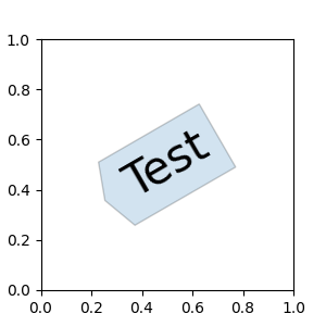
See also Custom box styles. Similarly, you can define a
custom ConnectionStyle and a custom ArrowStyle. View the source code at
patches to learn how each class is defined.
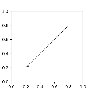
Customizing annotation arrows#
An arrow connecting xy to xytext can be optionally drawn by specifying the arrowprops argument. To draw only an arrow, use empty string as the first argument:
fig, ax = plt.subplots(figsize=(3, 3))
ax.annotate("",
            xy=(0.2, 0.2), xycoords='data',
            xytext=(0.8, 0.8), textcoords='data',
            arrowprops=dict(arrowstyle="->", connectionstyle="arc3"))
The arrow is drawn as follows:
A path connecting the two points is created, as specified by the connectionstyle parameter.
The path is clipped to avoid patches patchA and patchB, if these are set.
The path is further shrunk by shrinkA and shrinkB (in pixels).
The path is transmuted to an arrow patch, as specified by the arrowstyle parameter.
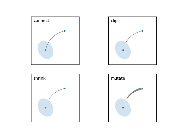
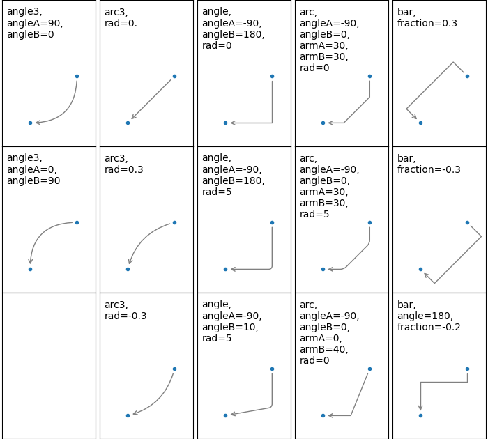
The creation of the connecting path between two points is controlled by
connectionstyle key and the following styles are available.
Name
Attrs
angleangleA=90,angleB=0,rad=0.0
angle3angleA=90,angleB=0
arcangleA=0,angleB=0,armA=None,armB=None,rad=0.0
arc3rad=0.0
bararmA=0.0,armB=0.0,fraction=0.3,angle=None
Note that "3" in angle3 and arc3 is meant to indicate that the
resulting path is a quadratic spline segment (three control
points). As will be discussed below, some arrow style options can only
be used when the connecting path is a quadratic spline.
The behavior of each connection style is (limitedly) demonstrated in the
example below. (Warning: The behavior of the bar style is currently not
well-defined and may be changed in the future).
The connecting path (after clipping and shrinking) is then mutated to
an arrow patch, according to the given arrowstyle.
Name
Attrs
-None
->head_length=0.4,head_width=0.2
-[widthB=1.0,lengthB=0.2,angleB=None
|-|widthA=1.0,widthB=1.0
-|>head_length=0.4,head_width=0.2
<-head_length=0.4,head_width=0.2
<->head_length=0.4,head_width=0.2
<|-head_length=0.4,head_width=0.2
<|-|>head_length=0.4,head_width=0.2
fancyhead_length=0.4,head_width=0.4,tail_width=0.4
simplehead_length=0.5,head_width=0.5,tail_width=0.2
wedgetail_width=0.3,shrink_factor=0.5
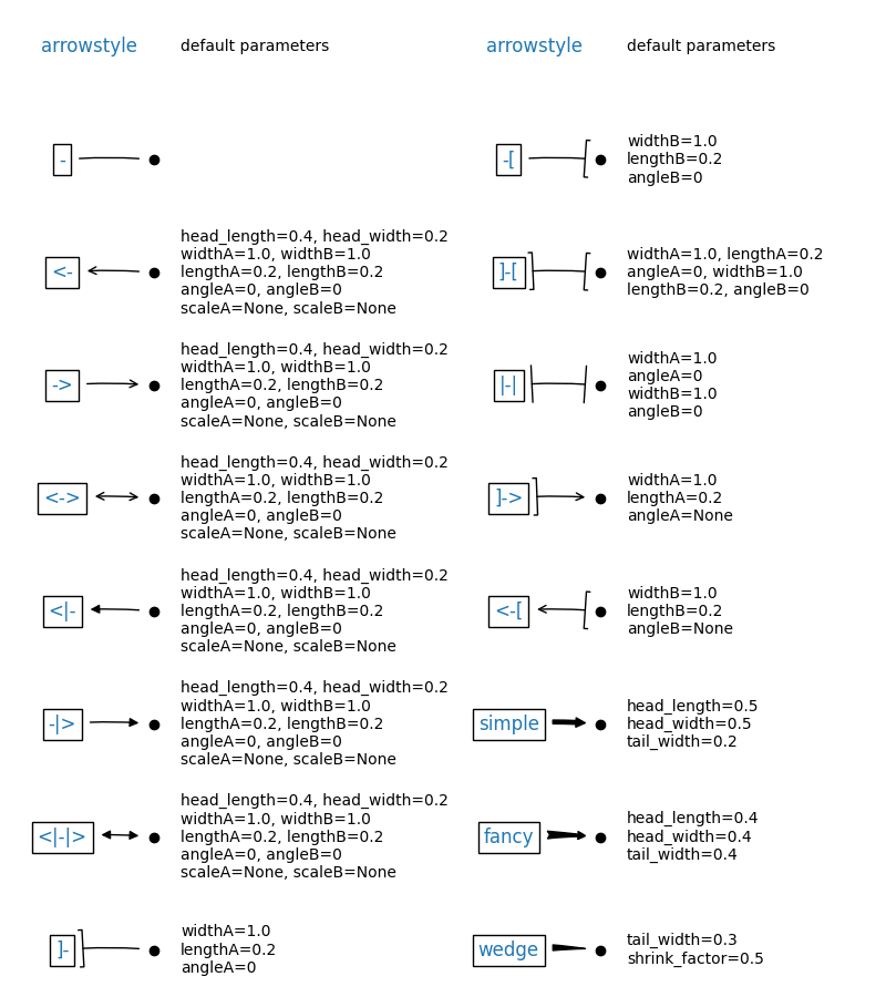
Some arrowstyles only work with connection styles that generate a
quadratic-spline segment. They are fancy, simple, and wedge.
For these arrow styles, you must use the "angle3" or "arc3" connection
style.
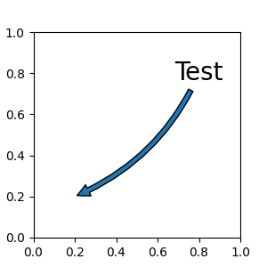
If the annotation string is given, the patch is set to the bbox patch of the text by default.
fig, ax = plt.subplots(figsize=(3, 3))

ax.annotate("Test",
            xy=(0.2, 0.2), xycoords='data',
            xytext=(0.8, 0.8), textcoords='data',
            size=20, va="center", ha="center",
            arrowprops=dict(arrowstyle="simple",
                            connectionstyle="arc3,rad=-0.2"))
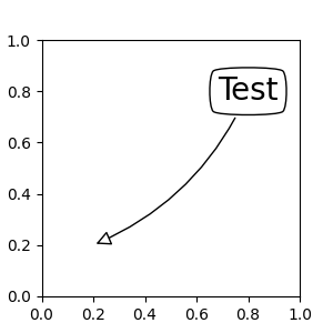
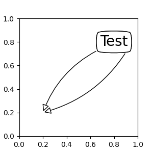
As with text, a box around the text can be drawn using the bbox
argument.
fig, ax = plt.subplots(figsize=(3, 3))

ann = ax.annotate("Test",
                  xy=(0.2, 0.2), xycoords='data',
                  xytext=(0.8, 0.8), textcoords='data',
                  size=20, va="center", ha="center",
                  bbox=dict(boxstyle="round4", fc="w"),
                  arrowprops=dict(arrowstyle="-|>",
                                  connectionstyle="arc3,rad=-0.2",
                                  fc="w"))
By default, the starting point is set to the center of the text
extent. This can be adjusted with relpos key value. The values
are normalized to the extent of the text. For example, (0, 0) means
lower-left corner and (1, 1) means top-right.
fig, ax = plt.subplots(figsize=(3, 3))

ann = ax.annotate("Test",
                  xy=(0.2, 0.2), xycoords='data',
                  xytext=(0.8, 0.8), textcoords='data',
                  size=20, va="center", ha="center",
                  bbox=dict(boxstyle="round4", fc="w"),
                  arrowprops=dict(arrowstyle="-|>",
                                  connectionstyle="arc3,rad=0.2",
                                  relpos=(0., 0.),
                                  fc="w"))

ann = ax.annotate("Test",
                  xy=(0.2, 0.2), xycoords='data',
                  xytext=(0.8, 0.8), textcoords='data',
                  size=20, va="center", ha="center",
                  bbox=dict(boxstyle="round4", fc="w"),
                  arrowprops=dict(arrowstyle="-|>",
                                  connectionstyle="arc3,rad=-0.2",
                                  relpos=(1., 0.),
                                  fc="w"))
Placing Artist at anchored Axes locations#
There are classes of artists that can be placed at an anchored
location in the Axes. A common example is the legend. This type
of artist can be created by using the OffsetBox class. A few
predefined classes are available in matplotlib.offsetbox and in
mpl_toolkits.axes_grid1.anchored_artists.
from matplotlib.offsetbox import AnchoredText

fig, ax = plt.subplots(figsize=(3, 3))
at = AnchoredText("Figure 1a",
                  prop=dict(size=15), frameon=True, loc='upper left')
at.patch.set_boxstyle("round,pad=0.,rounding_size=0.2")
ax.add_artist(at)
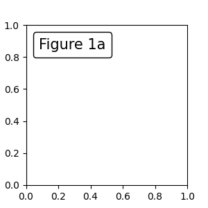
The loc keyword has same meaning as in the legend command.
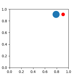
A simple application is when the size of the artist (or collection of
artists) is known in pixel size during the time of creation. For
example, If you want to draw a circle with fixed size of 20 pixel x 20
pixel (radius = 10 pixel), you can utilize
AnchoredDrawingArea. The instance
is created with a size of the drawing area (in pixels), and arbitrary artists
can be added to the drawing area. Note that the extents of the artists that are
added to the drawing area are not related to the placement of the drawing
area itself. Only the initial size matters.
The artists that are added to the drawing area should not have a transform set (it will be overridden) and the dimensions of those artists are interpreted as a pixel coordinate, i.e., the radius of the circles in above example are 10 pixels and 5 pixels, respectively.
from matplotlib.patches import Circle
from mpl_toolkits.axes_grid1.anchored_artists import AnchoredDrawingArea

fig, ax = plt.subplots(figsize=(3, 3))
ada = AnchoredDrawingArea(40, 20, 0, 0,
                          loc='upper right', pad=0., frameon=False)
p1 = Circle((10, 10), 10)
ada.drawing_area.add_artist(p1)
p2 = Circle((30, 10), 5, fc="r")
ada.drawing_area.add_artist(p2)
ax.add_artist(ada)
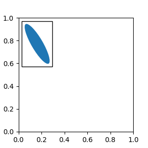
Sometimes, you want your artists to scale with the data coordinate (or
coordinates other than canvas pixels). You can use
AnchoredAuxTransformBox class.
This is similar to
AnchoredDrawingArea except that
the extent of the artist is determined during the drawing time respecting the
specified transform.
The ellipse in the example below will have width and height corresponding to 0.1 and 0.4 in data coordinates and will be automatically scaled when the view limits of the axes change.
from matplotlib.patches import Ellipse
from mpl_toolkits.axes_grid1.anchored_artists import AnchoredAuxTransformBox

fig, ax = plt.subplots(figsize=(3, 3))
box = AnchoredAuxTransformBox(ax.transData, loc='upper left')
el = Ellipse((0, 0), width=0.1, height=0.4, angle=30)  # in data coordinates!
box.drawing_area.add_artist(el)
ax.add_artist(box)
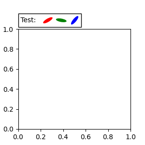
Another method of anchoring an artist relative to a parent axes or anchor
point is via the bbox_to_anchor argument of AnchoredOffsetbox. This
artist can then be automatically positioned relative to another artist using
HPacker and VPacker:
from matplotlib.offsetbox import (AnchoredOffsetbox, DrawingArea, HPacker,
                                  TextArea)

fig, ax = plt.subplots(figsize=(3, 3))

box1 = TextArea(" Test: ", textprops=dict(color="k"))
box2 = DrawingArea(60, 20, 0, 0)

el1 = Ellipse((10, 10), width=16, height=5, angle=30, fc="r")
el2 = Ellipse((30, 10), width=16, height=5, angle=170, fc="g")
el3 = Ellipse((50, 10), width=16, height=5, angle=230, fc="b")
box2.add_artist(el1)
box2.add_artist(el2)
box2.add_artist(el3)

box = HPacker(children=[box1, box2],
              align="center",
              pad=0, sep=5)

anchored_box = AnchoredOffsetbox(loc='lower left',
                                 child=box, pad=0.,
                                 frameon=True,
                                 bbox_to_anchor=(0., 1.02),
                                 bbox_transform=ax.transAxes,
                                 borderpad=0.,)

ax.add_artist(anchored_box)
fig.subplots_adjust(top=0.8)
Note that, unlike in Legend, the bbox_transform is set to
IdentityTransform by default
Coordinate systems for annotations#
Matplotlib Annotations support several types of coordinate systems. The
examples in Basic annotation used the data coordinate system;
Some others more advanced options are:
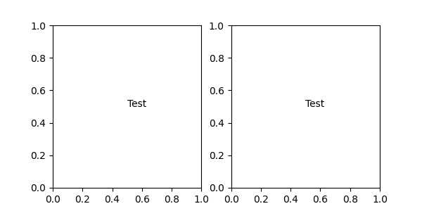
1. A Transform instance. For more information on transforms, see the
Transformations Tutorial For example, the
Axes.transAxes transform positions the annotation relative to the Axes
coordinates and using it is therefore identical to setting the
coordinate system to "axes fraction":
fig, (ax1, ax2) = plt.subplots(nrows=1, ncols=2, figsize=(6, 3))
ax1.annotate("Test", xy=(0.5, 0.5), xycoords=ax1.transAxes)
ax2.annotate("Test", xy=(0.5, 0.5), xycoords="axes fraction")
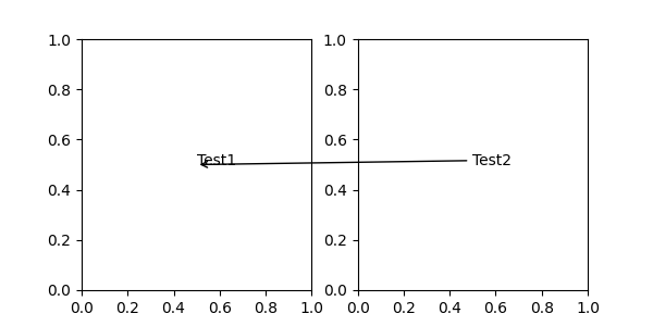
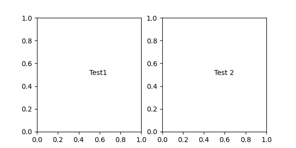
Another commonly used Transform instance is Axes.transData. This
transform is the coordinate system of the data plotted in the axes. In this
example, it is used to draw an arrow from a point in ax1 to text in ax2,
where the point and text are positioned relative to the coordinates of ax1
and ax2 respectively:
fig, (ax1, ax2) = plt.subplots(nrows=1, ncols=2, figsize=(6, 3))

ax1.annotate("Test1", xy=(0.5, 0.5), xycoords="axes fraction")
ax2.annotate("Test2",
               xy=(0.5, 0.5), xycoords=ax1.transData,
               xytext=(0.5, 0.5), textcoords=ax2.transData,
               arrowprops=dict(arrowstyle="->"))
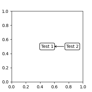
2. An Artist instance. The xy value (or xytext) is interpreted as a
fractional coordinate of the bounding box (bbox) of the artist:
fig, ax = plt.subplots(nrows=1, ncols=1, figsize=(3, 3))
an1 = ax.annotate("Test 1",
                  xy=(0.5, 0.5), xycoords="data",
                  va="center", ha="center",
                  bbox=dict(boxstyle="round", fc="w"))

an2 = ax.annotate("Test 2",
                  xy=(1, 0.5), xycoords=an1,  # (1, 0.5) of an1's bbox
                  xytext=(30, 0), textcoords="offset points",
                  va="center", ha="left",
                  bbox=dict(boxstyle="round", fc="w"),
                  arrowprops=dict(arrowstyle="->"))

Note that you must ensure that the extent of the coordinate artist (an1 in
this example) is determined before an2 gets drawn. Usually, this means
that an2 needs to be drawn after an1. The base class for all bounding
boxes is BboxBase
3. A callable object that takes the renderer instance as single argument, and
returns either a Transform or a BboxBase. For example, the return
value of Artist.get_window_extent is a bbox, so this method is identical
to (2) passing in the artist:
fig, ax = plt.subplots(nrows=1, ncols=1, figsize=(3, 3))
an1 = ax.annotate("Test 1",
                  xy=(0.5, 0.5), xycoords="data",
                  va="center", ha="center",
                  bbox=dict(boxstyle="round", fc="w"))

an2 = ax.annotate("Test 2",
                  xy=(1, 0.5), xycoords=an1.get_window_extent,
                  xytext=(30, 0), textcoords="offset points",
                  va="center", ha="left",
                  bbox=dict(boxstyle="round", fc="w"),
                  arrowprops=dict(arrowstyle="->"))
Artist.get_window_extent is the bounding box of the Axes object and is
therefore identical to setting the coordinate system to axes fraction:
fig, (ax1, ax2) = plt.subplots(nrows=1, ncols=2, figsize=(6, 3))

an1 = ax1.annotate("Test1", xy=(0.5, 0.5), xycoords="axes fraction")
an2 = ax2.annotate("Test 2", xy=(0.5, 0.5), xycoords=ax2.get_window_extent)
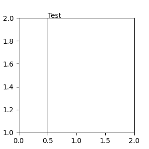
4. A blended pair of coordinate specifications -- the first for the x-coordinate, and the second is for the y-coordinate. For example, x=0.5 is in data coordinates, and y=1 is in normalized axes coordinates:
fig, ax = plt.subplots(figsize=(3, 3))
ax.annotate("Test", xy=(0.5, 1), xycoords=("data", "axes fraction"))
ax.axvline(x=.5, color='lightgray')
ax.set(xlim=(0, 2), ylim=(1, 2))
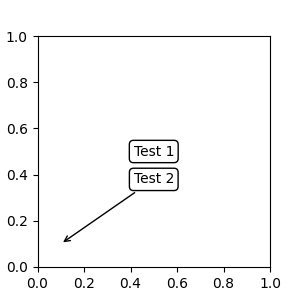
5. Sometimes, you want your annotation with some "offset points", not from the
annotated point but from some other point or artist. text.OffsetFrom is
a helper for such cases.
from matplotlib.text import OffsetFrom

fig, ax = plt.subplots(figsize=(3, 3))
an1 = ax.annotate("Test 1", xy=(0.5, 0.5), xycoords="data",
                  va="center", ha="center",
                  bbox=dict(boxstyle="round", fc="w"))

offset_from = OffsetFrom(an1, (0.5, 0))
an2 = ax.annotate("Test 2", xy=(0.1, 0.1), xycoords="data",
                  xytext=(0, -10), textcoords=offset_from,
                  # xytext is offset points from "xy=(0.5, 0), xycoords=an1"
                  va="top", ha="center",
                  bbox=dict(boxstyle="round", fc="w"),
                  arrowprops=dict(arrowstyle="->"))
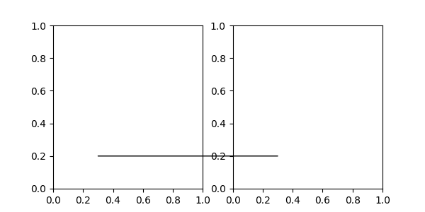
Using ConnectionPatch#
ConnectionPatch is like an annotation without text. While annotate
is sufficient in most situations, ConnectionPatch is useful when you want
to connect points in different axes. For example, here we connect the point
xy in the data coordinates of ax1 to point xy in the data coordinates
of ax2:
from matplotlib.patches import ConnectionPatch

fig, (ax1, ax2) = plt.subplots(nrows=1, ncols=2, figsize=(6, 3))
xy = (0.3, 0.2)
con = ConnectionPatch(xyA=xy, coordsA=ax1.transData,
                      xyB=xy, coordsB=ax2.transData)

fig.add_artist(con)
Here, we added the ConnectionPatch to the figure
(with add_artist) rather than to either axes. This ensures that
the ConnectionPatch artist is drawn on top of both axes, and is also necessary
when using constrained_layout for positioning the axes.
Zoom effect between Axes#
mpl_toolkits.axes_grid1.inset_locator defines some patch classes useful for
interconnecting two axes.
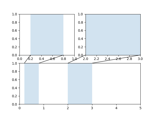
The code for this figure is at Axes Zoom Effect and familiarity with Transformations Tutorial is recommended.
Total running time of the script: ( 0 minutes 3.874 seconds)