What's new in Matplotlib 3.7.0 (Feb 13, 2023)#

For a list of all of the issues and pull requests since the last revision, see the GitHub statistics (Feb 13, 2023).

Plotting and Annotation improvements #

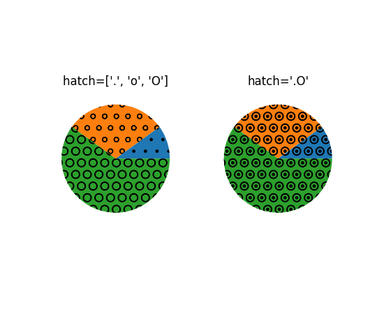
`hatch` parameter for pie #

pie now accepts a hatch keyword that takes as input a hatch or list of hatches:

fig, (ax1, ax2) = plt.subplots(ncols=2)
x = [10, 30, 60]

ax1.pie(x, hatch=['.', 'o', 'O'])
ax2.pie(x, hatch='.O')

ax1.set_title("hatch=['.', 'o', 'O']")
ax2.set_title("hatch='.O'")

(Source code, png)

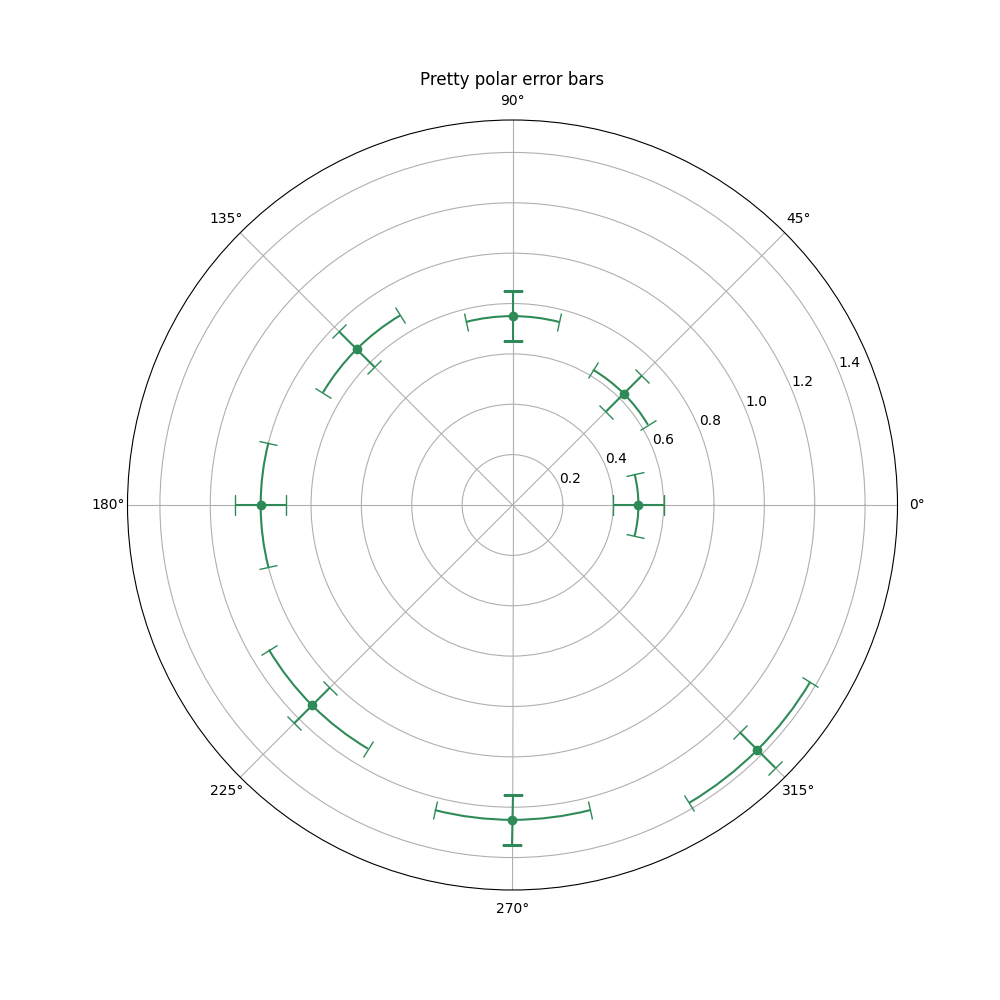
Two pie charts, identified as ax1 and ax2, both have a small blue slice, a medium orange slice, and a large green slice. ax1 has a dot hatching on the small slice, a small open circle hatching on the medium slice, and a large open circle hatching on the large slice. ax2 has the same large open circle with a dot hatch on every slice.

Polar plot errors drawn in polar coordinates #

Caps and error lines are now drawn with respect to polar coordinates, when plotting errorbars on polar plots.

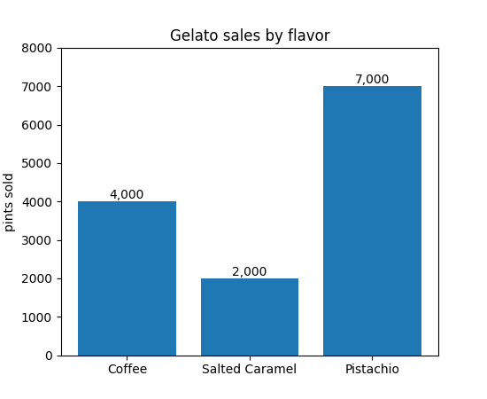
../../_images/sphx_glr_polar_error_caps_001.png

Additional format string options in `bar_label`#

The fmt argument of bar_label now accepts {}-style format strings:

import matplotlib.pyplot as plt

fruit_names = ['Coffee', 'Salted Caramel', 'Pistachio']
fruit_counts = [4000, 2000, 7000]

fig, ax = plt.subplots()
bar_container = ax.bar(fruit_names, fruit_counts)
ax.set(ylabel='pints sold', title='Gelato sales by flavor', ylim=(0, 8000))
ax.bar_label(bar_container, fmt='{:,.0f}')

(Source code, png)

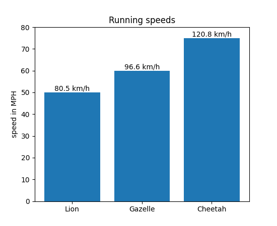
It also accepts callables:

animal_names = ['Lion', 'Gazelle', 'Cheetah']
mph_speed = [50, 60, 75]

fig, ax = plt.subplots()
bar_container = ax.bar(animal_names, mph_speed)
ax.set(ylabel='speed in MPH', title='Running speeds', ylim=(0, 80))
ax.bar_label(
    bar_container, fmt=lambda x: '{:.1f} km/h'.format(x * 1.61)
)

(Source code, png)

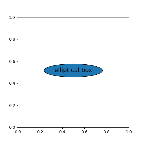
`ellipse` boxstyle option for annotations #

The 'ellipse' option for boxstyle can now be used to create annotations with an elliptical outline. It can be used as a closed curve shape for longer texts instead of the 'circle' boxstyle which can get quite big.

import matplotlib.pyplot as plt
fig, ax = plt.subplots(figsize=(5, 5))
t = ax.text(0.5, 0.5, "elliptical box",
        ha="center", size=15,
        bbox=dict(boxstyle="ellipse,pad=0.3"))

(Source code, png)

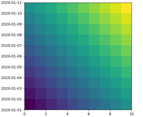
The extent of `imshow` can now be expressed with units #

The extent parameter of imshow and set_extent can now be expressed with units.

import matplotlib.pyplot as plt
import numpy as np

fig, ax = plt.subplots(layout='constrained')
date_first = np.datetime64('2020-01-01', 'D')
date_last = np.datetime64('2020-01-11', 'D')

arr = [[i+j for i in range(10)] for j in range(10)]

ax.imshow(arr, origin='lower', extent=[0, 10, date_first, date_last])

plt.show()

(Source code, png)

Reversed order of legend entries #

The order of legend entries can now be reversed by passing reverse=True to legend.

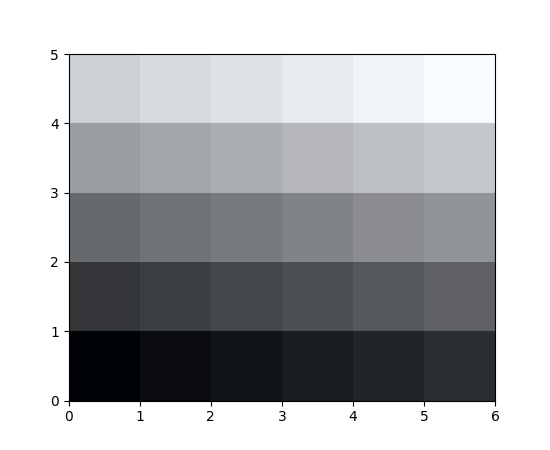
`pcolormesh` accepts RGB(A) colors #

The pcolormesh method can now handle explicit colors specified with RGB(A) values. To specify colors, the array must be 3D with a shape of (M, N, [3, 4]).

import matplotlib.pyplot as plt
import numpy as np

colors = np.linspace(0, 1, 90).reshape((5, 6, 3))
plt.pcolormesh(colors)
plt.show()

(Source code, png)

View current appearance settings for ticks, tick labels, and gridlines #

The new get_tick_params method can be used to retrieve the appearance settings that will be applied to any additional ticks, tick labels, and gridlines added to the plot:

>>> import matplotlib.pyplot as plt

>>> fig, ax = plt.subplots()
>>> ax.yaxis.set_tick_params(labelsize=30, labelcolor='red',
...                          direction='out', which='major')
>>> ax.yaxis.get_tick_params(which='major')
{'direction': 'out',
'left': True,
'right': False,
'labelleft': True,
'labelright': False,
'gridOn': False,
'labelsize': 30,
'labelcolor': 'red'}
>>> ax.yaxis.get_tick_params(which='minor')
{'left': True,
'right': False,
'labelleft': True,
'labelright': False,
'gridOn': False}

Style files can be imported from third-party packages #

Third-party packages can now distribute style files that are globally available as follows. Assume that a package is importable as import mypackage, with a mypackage/__init__.py module. Then a mypackage/presentation.mplstyle style sheet can be used as plt.style.use("mypackage.presentation").

The implementation does not actually import mypackage, making this process safe against possible import-time side effects. Subpackages (e.g. dotted.package.name) are also supported.

Improvements to 3D Plotting #

3D plot pan and zoom buttons #

The pan and zoom buttons in the toolbar of 3D plots are now enabled. Unselect both to rotate the plot. When the zoom button is pressed, zoom in by using the left mouse button to draw a bounding box, and out by using the right mouse button to draw the box. When zooming a 3D plot, the current view aspect ratios are kept fixed.

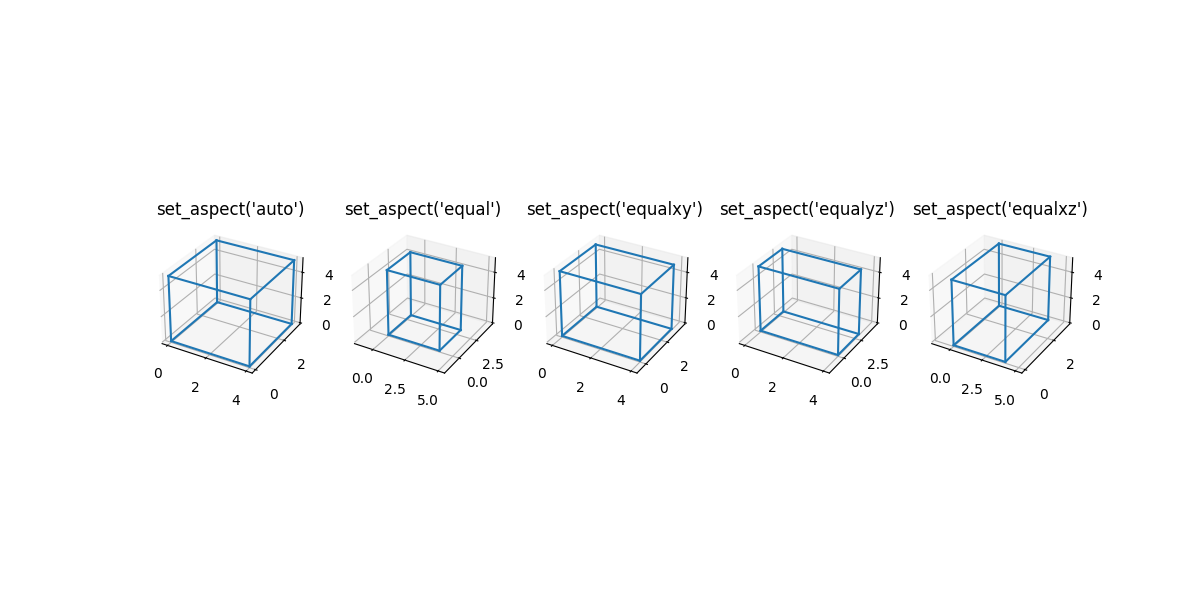
adjustable keyword argument for setting equal aspect ratios in 3D #

While setting equal aspect ratios for 3D plots, users can choose to modify either the data limits or the bounding box in parity with 2D Axes.

import matplotlib.pyplot as plt
import numpy as np
from itertools import combinations, product

aspects = ('auto', 'equal', 'equalxy', 'equalyz', 'equalxz')
fig, axs = plt.subplots(1, len(aspects), subplot_kw={'projection': '3d'},
                        figsize=(12, 6))

# Draw rectangular cuboid with side lengths [4, 3, 5]
r = [0, 1]
scale = np.array([4, 3, 5])
pts = combinations(np.array(list(product(r, r, r))), 2)
for start, end in pts:
    if np.sum(np.abs(start - end)) == r[1] - r[0]:
        for ax in axs:
            ax.plot3D(*zip(start*scale, end*scale), color='C0')

# Set the aspect ratios
for i, ax in enumerate(axs):
    ax.set_aspect(aspects[i], adjustable='datalim')
    # Alternatively: ax.set_aspect(aspects[i], adjustable='box')
    # which will change the box aspect ratio instead of axis data limits.
    ax.set_title(f"set_aspect('{aspects[i]}')")

plt.show()

(Source code, png)

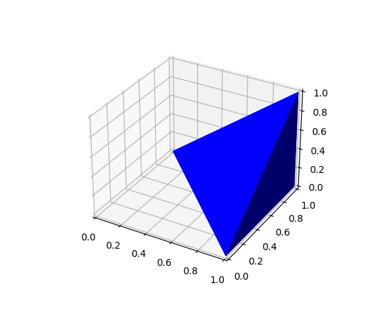
`Poly3DCollection` supports shading #

It is now possible to shade a Poly3DCollection. This is useful if the polygons are obtained from e.g. a 3D model.

import numpy as np
import matplotlib.pyplot as plt
from mpl_toolkits.mplot3d.art3d import Poly3DCollection

# Define 3D shape
block = np.array([
    [[1, 1, 0],
     [1, 0, 0],
     [0, 1, 0]],
    [[1, 1, 0],
     [1, 1, 1],
     [1, 0, 0]],
    [[1, 1, 0],
     [1, 1, 1],
     [0, 1, 0]],
    [[1, 0, 0],
     [1, 1, 1],
     [0, 1, 0]]
])

ax = plt.subplot(projection='3d')
pc = Poly3DCollection(block, facecolors='b', shade=True)
ax.add_collection(pc)
plt.show()

(Source code, png)

rcParam for 3D pane color #

The rcParams rcParams["axes3d.xaxis.panecolor"] (default: (0.95, 0.95, 0.95, 0.5)), rcParams["axes3d.yaxis.panecolor"] (default: (0.9, 0.9, 0.9, 0.5)), rcParams["axes3d.zaxis.panecolor"] (default: (0.925, 0.925, 0.925, 0.5)) can be used to change the color of the background panes in 3D plots. Note that it is often beneficial to give them slightly different shades to obtain a "3D effect" and to make them slightly transparent (alpha < 1).

import matplotlib.pyplot as plt
with plt.rc_context({'axes3d.xaxis.panecolor': (0.9, 0.0, 0.0, 0.5),
                     'axes3d.yaxis.panecolor': (0.7, 0.0, 0.0, 0.5),
                     'axes3d.zaxis.panecolor': (0.8, 0.0, 0.0, 0.5)}):
    fig = plt.figure()
    fig.add_subplot(projection='3d')

(Source code, png)

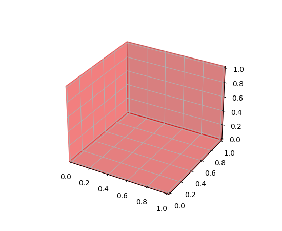
Figure and Axes Layout #

`colorbar` now has a location keyword argument #

The colorbar method now supports a location keyword argument to more easily position the color bar. This is useful when providing your own inset axes using the cax keyword argument and behaves similar to the case where axes are not provided (where the location keyword is passed through). orientation and ticklocation are no longer required as they are determined by location. ticklocation can still be provided if the automatic setting is not preferred. (orientation can also be provided but must be compatible with the location.)

An example is:

import matplotlib.pyplot as plt
import numpy as np
rng = np.random.default_rng(19680801)
imdata = rng.random((10, 10))
fig, ax = plt.subplots(layout='constrained')
im = ax.imshow(imdata)
fig.colorbar(im, cax=ax.inset_axes([0, 1.05, 1, 0.05]),
             location='top')

(Source code, png)

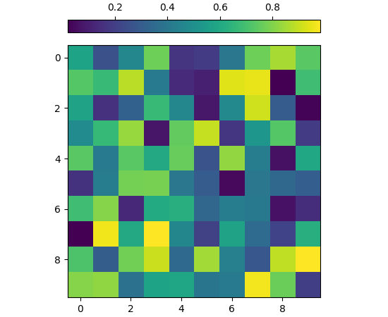
Figure legends can be placed outside figures using constrained_layout #

Constrained layout will make space for Figure legends if they are specified by a loc keyword argument that starts with the string "outside". The codes are unique from axes codes, in that "outside upper right" will make room at the top of the figure for the legend, whereas "outside right upper" will make room on the right-hand side of the figure. See Legend guide for details.

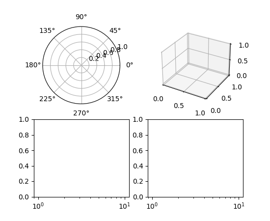
Per-subplot keyword arguments in `subplot_mosaic`#

It is now possible to pass keyword arguments through to Axes creation in each specific call to add_subplot in Figure.subplot_mosaic and pyplot.subplot_mosaic :

fig, axd = plt.subplot_mosaic(
    "AB;CD",
    per_subplot_kw={
        "A": {"projection": "polar"},
        ("C", "D"): {"xscale": "log"},
        "B": {"projection": "3d"},
    },
)

(Source code, png)

This is particularly useful for creating mosaics with mixed projections, but any keyword arguments can be passed through.

`subplot_mosaic` no longer provisional #

The API on Figure.subplot_mosaic and pyplot.subplot_mosaic are now considered stable and will change under Matplotlib's normal deprecation process.

Widget Improvements #

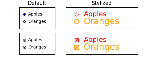
Custom styling of button widgets #

Additional custom styling of button widgets may be achieved via the label_props and radio_props arguments to RadioButtons; and the label_props, frame_props, and check_props arguments to CheckButtons.

(Source code, png)

Blitting in Button widgets #

The Button, CheckButtons, and RadioButtons widgets now support blitting for faster rendering, on backends that support it, by passing useblit=True to the constructor. Blitting is enabled by default on supported backends.

Other Improvements #

Source links can be shown or hidden for each Sphinx plot directive #

The Sphinx plot directive (.. plot::) now supports a :show-source-link: option to show or hide the link to the source code for each plot. The default is set using the plot_html_show_source_link variable in conf.py (which defaults to True).

Figure hooks #

The new rcParams["figure.hooks"] (default: []) provides a mechanism to register arbitrary customizations on pyplot figures; it is a list of "dotted.module.name:dotted.callable.name" strings specifying functions that are called on each figure created by pyplot.figure; these functions can e.g. attach callbacks or modify the toolbar. See mplcvd -- an example of figure hook for an example of toolbar customization.

New & Improved Narrative Documentation #

Brand new Animations tutorial.
New grouped and stacked bar chart examples.
New section for new contributors and reorganized git instructions in the contributing guide.
Restructured Annotations tutorial.