Version 3.1.2
Note
Click here to download the full example code
Demonstrate the Sankey class by producing three basic diagrams.
import matplotlib.pyplot as plt

from matplotlib.sankey import Sankey
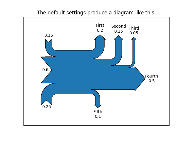
Example 1 -- Mostly defaults
This demonstrates how to create a simple diagram by implicitly calling the Sankey.add() method and by appending finish() to the call to the class.
Out:
Text(0.5, 1.0, 'The default settings produce a diagram like this.')
Notice:
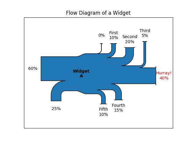
Example 2
This demonstrates:
fig = plt.figure()
ax = fig.add_subplot(1, 1, 1, xticks=[], yticks=[],
                     title="Flow Diagram of a Widget")
sankey = Sankey(ax=ax, scale=0.01, offset=0.2, head_angle=180,
                format='%.0f', unit='%')
sankey.add(flows=[25, 0, 60, -10, -20, -5, -15, -10, -40],
           labels=['', '', '', 'First', 'Second', 'Third', 'Fourth',
                   'Fifth', 'Hurray!'],
           orientations=[-1, 1, 0, 1, 1, 1, -1, -1, 0],
           pathlengths=[0.25, 0.25, 0.25, 0.25, 0.25, 0.6, 0.25, 0.25,
                        0.25],
           patchlabel="Widget\nA")  # Arguments to matplotlib.patches.PathPatch()
diagrams = sankey.finish()
diagrams[0].texts[-1].set_color('r')
diagrams[0].text.set_fontweight('bold')
Notice:
Example 3
This demonstrates:
fig = plt.figure()
ax = fig.add_subplot(1, 1, 1, xticks=[], yticks=[], title="Two Systems")
flows = [0.25, 0.15, 0.60, -0.10, -0.05, -0.25, -0.15, -0.10, -0.35]
sankey = Sankey(ax=ax, unit=None)
sankey.add(flows=flows, label='one',
           orientations=[-1, 1, 0, 1, 1, 1, -1, -1, 0])
sankey.add(flows=[-0.25, 0.15, 0.1], label='two',
           orientations=[-1, -1, -1], prior=0, connect=(0, 0))
diagrams = sankey.finish()
diagrams[-1].patch.set_hatch('/')
plt.legend()
Out:
<matplotlib.legend.Legend object at 0x7fb113d392e8>
Notice that only one connection is specified, but the systems form a circuit since: (1) the lengths of the paths are justified and (2) the orientation and ordering of the flows is mirrored.
plt.show()
The use of the following functions, methods, classes and modules is shown in this example:
import matplotlib
matplotlib.sankey
matplotlib.sankey.Sankey
matplotlib.sankey.Sankey.add
matplotlib.sankey.Sankey.finish
Out:
<function Sankey.finish at 0x7fb11a993510>
Keywords: matplotlib code example, codex, python plot, pyplot Gallery generated by Sphinx-Gallery