Version 3.1.2
Note
Click here to download the full example code
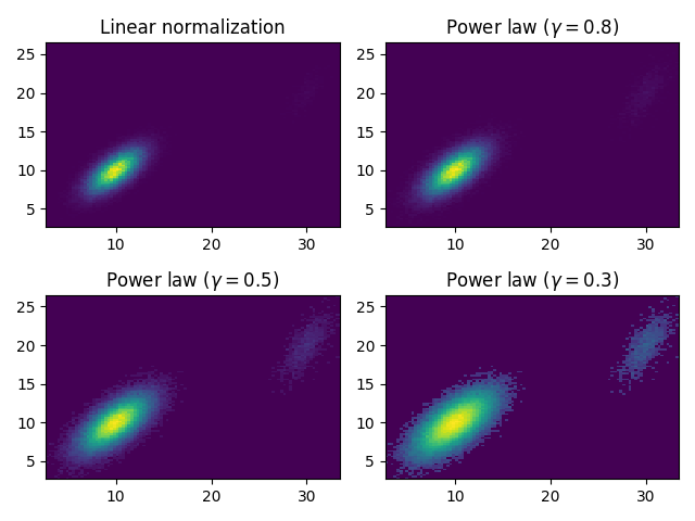
Various normalization on a multivariate normal distribution.
import matplotlib.pyplot as plt
import matplotlib.colors as mcolors
import numpy as np
from numpy.random import multivariate_normal

data = np.vstack([
    multivariate_normal([10, 10], [[3, 2], [2, 3]], size=100000),
    multivariate_normal([30, 20], [[2, 3], [1, 3]], size=1000)
])

gammas = [0.8, 0.5, 0.3]

fig, axes = plt.subplots(nrows=2, ncols=2)

axes[0, 0].set_title('Linear normalization')
axes[0, 0].hist2d(data[:, 0], data[:, 1], bins=100)

for ax, gamma in zip(axes.flat[1:], gammas):
    ax.set_title(r'Power law $(\gamma=%1.1f)$' % gamma)
    ax.hist2d(data[:, 0], data[:, 1],
              bins=100, norm=mcolors.PowerNorm(gamma))

fig.tight_layout()

plt.show()
The use of the following functions, methods, classes and modules is shown in this example:
import matplotlib
matplotlib.colors
matplotlib.colors.PowerNorm
matplotlib.axes.Axes.hist2d
matplotlib.pyplot.hist2d
Out:
<function hist2d at 0x7fb11b162620>
Keywords: matplotlib code example, codex, python plot, pyplot Gallery generated by Sphinx-Gallery