Version 2.2.2
Note
Click here to download the full example code
How to use constrained-layout to fit plots within your figure cleanly.
constrained_layout automatically adjusts subplots and decorations like legends and colorbars so that they fit in the figure window while still preserving, as best they can, the logical layout requested by the user.
constrained_layout is similar to tight_layout, but uses a constraint solver to determine the size of axes that allows them to fit.
Warning
As of Matplotlib 2.2, Constrained Layout is experimental. The
behaviour and API are subject to change, or the whole functionality
may be removed without a deprecation period. If you require your
plots to be absolutely reproducible, get the Axes positions after
running Constrained Layout and use ax.set_position() in your code
with constrained_layout=False.
In Matplotlib, the location of axes (including subplots) are specified in normalized figure coordinates. It can happen that your axis labels or titles (or sometimes even ticklabels) go outside the figure area, and are thus clipped.
# sphinx_gallery_thumbnail_number = 18

#import matplotlib
#matplotlib.use('Qt5Agg')

import warnings

import matplotlib.pyplot as plt
import numpy as np
import matplotlib.colors as mcolors
import matplotlib.gridspec as gridspec

import matplotlib._layoutbox as layoutbox

plt.rcParams['savefig.facecolor'] = "0.8"
plt.rcParams['figure.figsize'] = 4.5, 4.


def example_plot(ax, fontsize=12, nodec=False):
    ax.plot([1, 2])

    ax.locator_params(nbins=3)
    if not nodec:
        ax.set_xlabel('x-label', fontsize=fontsize)
        ax.set_ylabel('y-label', fontsize=fontsize)
        ax.set_title('Title', fontsize=fontsize)
    else:
        ax.set_xticklabels('')
        ax.set_yticklabels('')


fig, ax = plt.subplots()
example_plot(ax, fontsize=24)
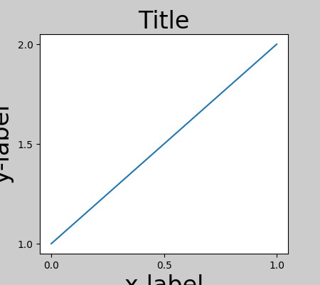
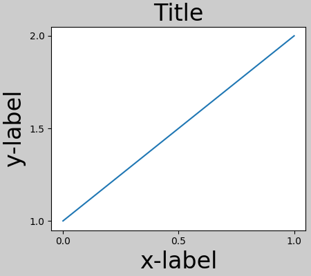
To prevent this, the location of axes needs to be adjusted. For
subplots, this can be done by adjusting the subplot params
(Move the edge of an axes to make room for tick labels). However, specifying your figure with the
constrained_layout=True kwarg will do the adjusting automatically.
fig, ax = plt.subplots(constrained_layout=True)
example_plot(ax, fontsize=24)
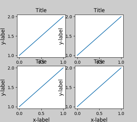
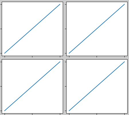
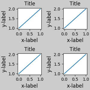
When you have multiple subplots, often you see labels of different axes overlapping each other.
fig, axs = plt.subplots(2, 2, constrained_layout=False)
for ax in axs.flatten():
    example_plot(ax)
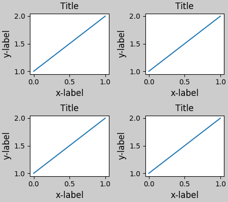
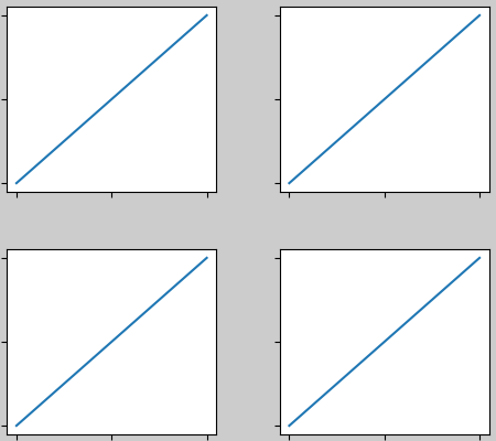
Specifying constrained_layout=True in the call to plt.subplots
causes the layout to be properly constrained.
fig, axs = plt.subplots(2, 2, constrained_layout=True)
for ax in axs.flatten():
    example_plot(ax)
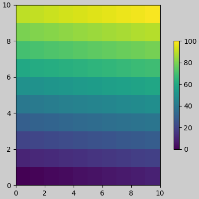
If you create a colorbar with the colorbar()
command you need to make room for it. constrained_layout does this
automatically. Note that if you specify use_gridspec=True it will be
ignored because this option is made for improving the layout via
tight_layout.
Note
For the pcolormesh kwargs (pc_kwargs) we use a dictionary.
Below we will assign one colorbar to a number of axes each containing
a ScalarMappable; specifying the norm and colormap ensures
the colorbar is accurate for all the axes.
arr = np.arange(100).reshape((10, 10))
norm = mcolors.Normalize(vmin=0., vmax=100.)
# see note above: this makes all pcolormesh calls consistent:
pc_kwargs = {'rasterized':True, 'cmap':'viridis', 'norm':norm}
fig, ax = plt.subplots(figsize=(4, 4), constrained_layout=True)
im = ax.pcolormesh(arr, **pc_kwargs)
fig.colorbar(im, ax=ax, shrink=0.6)
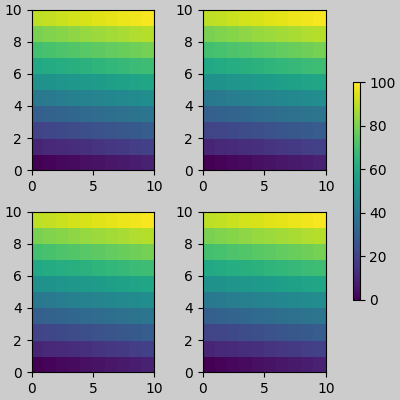
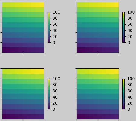
If you specify a list of axes (or other iterable container) to the
ax argument of colorbar, constrained_layout will take space from all # axes that share the same gridspec.
fig, axs = plt.subplots(2, 2, figsize=(4, 4), constrained_layout=True)
for ax in axs.flatten():
    im = ax.pcolormesh(arr, **pc_kwargs)
fig.colorbar(im, ax=axs, shrink=0.6)
Note that there is a bit of a subtlety when specifying a single axes as the parent. In the following, it might be desirable and expected for the colorbars to line up, but they don’t because the colorbar paired with the bottom axes is tied to the subplotspec of the axes, and hence shrinks when the gridspec-level colorbar is added.
fig, axs = plt.subplots(3, 1, figsize=(4, 4), constrained_layout=True)
for ax in axs[:2]:
    im = ax.pcolormesh(arr, **pc_kwargs)
fig.colorbar(im, ax=axs[:2], shrink=0.6)
im = axs[2].pcolormesh(arr, **pc_kwargs)
fig.colorbar(im, ax=axs[2], shrink=0.6)
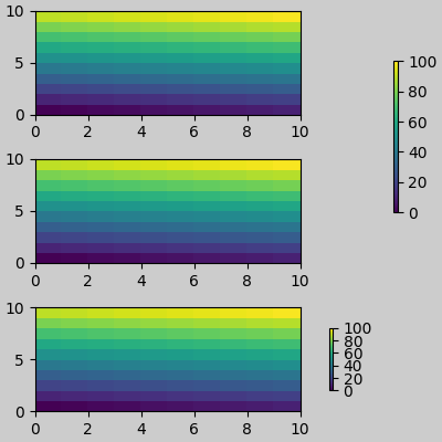
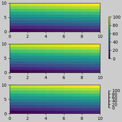
The API to make a single-axes behave like a list of axes is to specify it as a list (or other iterable container), as below:
fig, axs = plt.subplots(3, 1, figsize=(4, 4), constrained_layout=True)
for ax in axs[:2]:
    im = ax.pcolormesh(arr, **pc_kwargs)
fig.colorbar(im, ax=axs[:2], shrink=0.6)
im = axs[2].pcolormesh(arr, **pc_kwargs)
fig.colorbar(im, ax=[axs[2]], shrink=0.6)
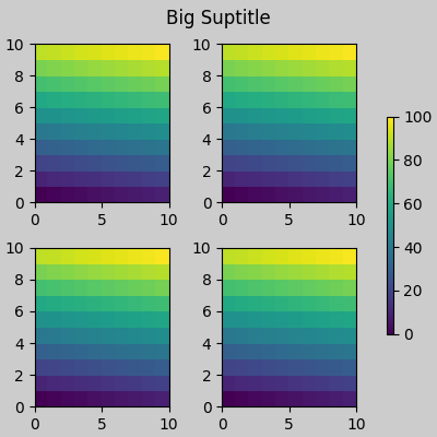
constrained_layout can also make room for suptitle.
fig, axs = plt.subplots(2, 2, figsize=(4, 4), constrained_layout=True)
for ax in axs.flatten():
    im = ax.pcolormesh(arr, **pc_kwargs)
fig.colorbar(im, ax=axs, shrink=0.6)
fig.suptitle('Big Suptitle')
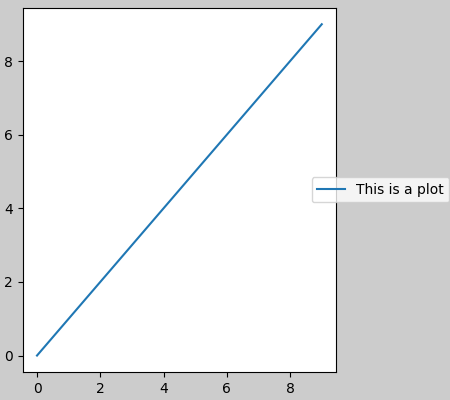
Legends can be placed outside
of their parent axis. Constrained-layout is designed to handle this.
However, constrained-layout does not handle legends being created via
fig.legend() (yet).
fig, ax = plt.subplots(constrained_layout=True)
ax.plot(np.arange(10), label='This is a plot')
ax.legend(loc='center left', bbox_to_anchor=(0.9, 0.5))
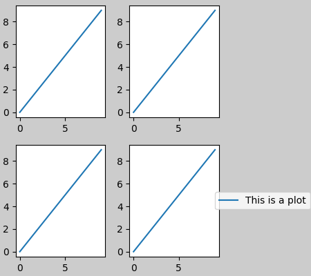
However, this will steal space from a subplot layout:
fig, axs = plt.subplots(2, 2, constrained_layout=True)
for ax in axs.flatten()[:-1]:
    ax.plot(np.arange(10))
axs[1, 1].plot(np.arange(10), label='This is a plot')
axs[1, 1].legend(loc='center left', bbox_to_anchor=(0.9, 0.5))
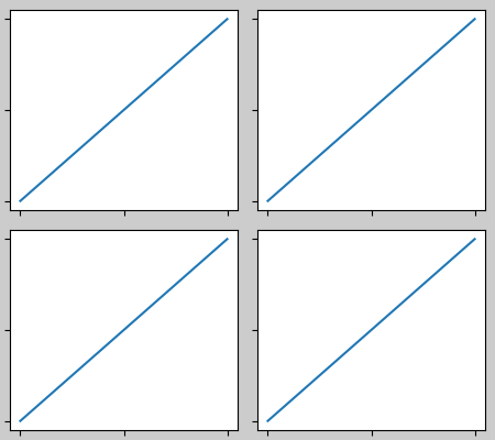
For constrained_layout, we have implemented a padding around the edge of
each axes. This padding sets the distance from the edge of the plot,
and the minimum distance between adjacent plots. It is specified in
inches by the keyword arguments w_pad and h_pad to the function
fig.set_constrained_layout_pads:
fig, axs = plt.subplots(2, 2, constrained_layout=True)
for ax in axs.flatten():
    example_plot(ax, nodec=True)
    ax.set_xticklabels('')
    ax.set_yticklabels('')
fig.set_constrained_layout_pads(w_pad=4./72., h_pad=4./72.,
        hspace=0., wspace=0.)

fig, axs = plt.subplots(2, 2, constrained_layout=True)
for ax in axs.flatten():
    example_plot(ax, nodec=True)
    ax.set_xticklabels('')
    ax.set_yticklabels('')
fig.set_constrained_layout_pads(w_pad=2./72., h_pad=2./72.,
        hspace=0., wspace=0.)
Spacing between subplots is set by wspace and hspace. There are
specified as a fraction of the size of the subplot group as a whole.
If the size of the figure is changed, then these spaces change in
proportion. Note in the blow how the space at the edges doesn’t change from
the above, but the space between subplots does.
fig, axs = plt.subplots(2, 2, constrained_layout=True)
for ax in axs.flatten():
    example_plot(ax, nodec=True)
    ax.set_xticklabels('')
    ax.set_yticklabels('')
fig.set_constrained_layout_pads(w_pad=2./72., h_pad=2./72.,
        hspace=0.2, wspace=0.2)
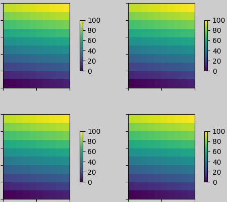
Colorbars still respect the w_pad and h_pad values. However they will
be wspace and hsapce apart from other subplots. Note the use of a pad
kwarg here in the colorbar call. It defaults to 0.02 of the size of the
axis it is attached to.
fig, axs = plt.subplots(2, 2, constrained_layout=True)
for ax in axs.flatten():
    pc = ax.pcolormesh(arr, **pc_kwargs)
    fig.colorbar(im, ax=ax, shrink=0.6, pad=0)
    ax.set_xticklabels('')
    ax.set_yticklabels('')
fig.set_constrained_layout_pads(w_pad=2./72., h_pad=2./72.,
        hspace=0.2, wspace=0.2)
In the above example, the colorbar will not ever be closer than 2 pts to
the plot, but if we want it a bit further away, we can specify its value
for pad to be non-zero.
fig, axs = plt.subplots(2, 2, constrained_layout=True)
for ax in axs.flatten():
    pc = ax.pcolormesh(arr, **pc_kwargs)
    fig.colorbar(im, ax=ax, shrink=0.6, pad=0.05)
    ax.set_xticklabels('')
    ax.set_yticklabels('')
fig.set_constrained_layout_pads(w_pad=2./72., h_pad=2./72.,
        hspace=0.2, wspace=0.2)
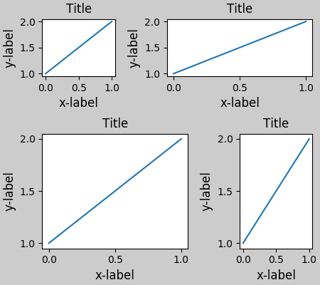
There are five rcParams that can be set, either in a script
or in the matplotlibrc file. They all have the prefix
figure.constrained_layout:
use: Whether to use constrained_layout. Default is Falsew_pad, h_pad Padding around axes objects.wspace, hspace Space between subplot groups.plt.rcParams['figure.constrained_layout.use'] = True
fig, axs = plt.subplots(2, 2, figsize=(3, 3))
for ax in axs.flatten():
example_plot(ax)
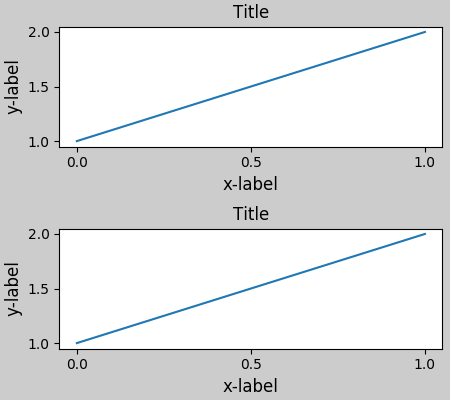
constrained_layout is meant to be used
with subplots() or
GridSpec() and
add_subplot().
fig = plt.figure(constrained_layout=True)

gs1 = gridspec.GridSpec(2, 1, figure=fig)
ax1 = fig.add_subplot(gs1[0])
ax2 = fig.add_subplot(gs1[1])

example_plot(ax1)
example_plot(ax2)
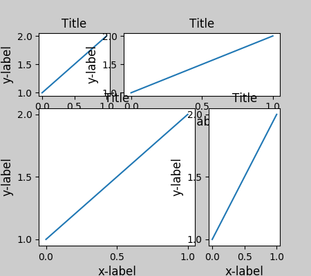
More complicated gridspec layouts are possible…
fig = plt.figure(constrained_layout=True)

gs0 = gridspec.GridSpec(1, 2, figure=fig)

gs1 = gridspec.GridSpecFromSubplotSpec(2, 1, gs0[0])
ax1 = fig.add_subplot(gs1[0])
ax2 = fig.add_subplot(gs1[1])

example_plot(ax1)
example_plot(ax2)

gs2 = gridspec.GridSpecFromSubplotSpec(3, 1, gs0[1])

for ss in gs2:
    ax = fig.add_subplot(ss)
    example_plot(ax)
    ax.set_title("")
    ax.set_xlabel("")

ax.set_xlabel("x-label", fontsize=12)
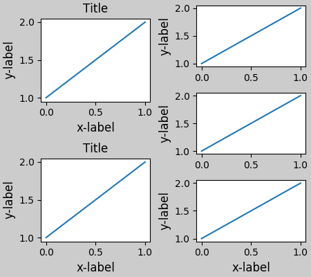
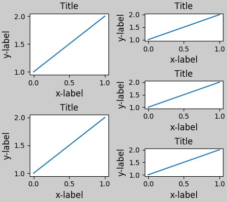
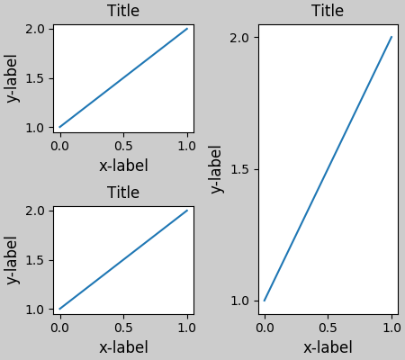
Note that in the above the left and columns don’t have the same vertical extent. If we want the top and bottom of the two grids to line up then they need to be in the same gridspec:
fig = plt.figure(constrained_layout=True)

gs0 = gridspec.GridSpec(6, 2, figure=fig)

ax1 = fig.add_subplot(gs0[:3, 0])
ax2 = fig.add_subplot(gs0[3:, 0])

example_plot(ax1)
example_plot(ax2)

ax = fig.add_subplot(gs0[0:2, 1])
example_plot(ax)
ax = fig.add_subplot(gs0[2:4, 1])
example_plot(ax)
ax = fig.add_subplot(gs0[4:, 1])
example_plot(ax)
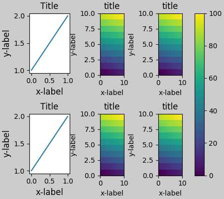
This example uses two gridspecs to have the colorbar only pertain to one set of pcolors. Note how the left column is wider than the two right-hand columns because of this. Of course, if you wanted the subplots to be the same size you only needed one gridspec.
def docomplicated(suptitle=None):
    fig = plt.figure(constrained_layout=True)
    gs0 = gridspec.GridSpec(1, 2, figure=fig, width_ratios=[1., 2.])
    gsl = gridspec.GridSpecFromSubplotSpec(2, 1, gs0[0])
    gsr = gridspec.GridSpecFromSubplotSpec(2, 2, gs0[1])

    for gs in gsl:
        ax = fig.add_subplot(gs)
        example_plot(ax)
    axs = []
    for gs in gsr:
        ax = fig.add_subplot(gs)
        pcm = ax.pcolormesh(arr, **pc_kwargs)
        ax.set_xlabel('x-label')
        ax.set_ylabel('y-label')
        ax.set_title('title')

        axs += [ax]
    fig.colorbar(pcm, ax=axs)
    if suptitle is not None:
        fig.suptitle(suptitle)

docomplicated()
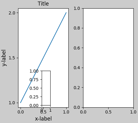
There can be good reasons to manually set an axes position. A manual call
to ax.set_position() will set the axes so constrained_layout has no
effect on it anymore. (Note that constrained_layout still leaves the space
for the axes that is moved).
fig, axs = plt.subplots(1, 2, constrained_layout=True)
example_plot(axs[0], fontsize=12)
axs[1].set_position([0.2, 0.2, 0.4, 0.4])
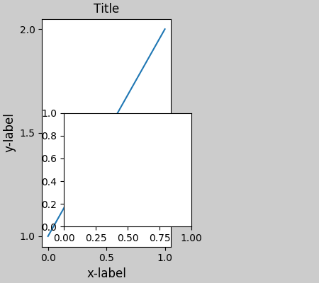
If you want an inset axes in data-space, you need to manually execute the
layout using fig.execute_constrained_layout() call. The inset figure
will then be properly positioned. However, it will not be properly
positioned if the size of the figure is subsequently changed. Similarly,
if the figure is printed to another backend, there may be slight changes
of location due to small differences in how the backends render fonts.
from matplotlib.transforms import Bbox

fig, axs = plt.subplots(1, 2, constrained_layout=True)
example_plot(axs[0], fontsize=12)
fig.execute_constrained_layout()
# put into data-space:
bb_data_ax2 = Bbox.from_bounds(0.5, 1., 0.2, 0.4)
disp_coords = axs[0].transData.transform(bb_data_ax2)
fig_coords_ax2 = fig.transFigure.inverted().transform(disp_coords)
bb_ax2 = Bbox(fig_coords_ax2)
ax2 = fig.add_axes(bb_ax2)
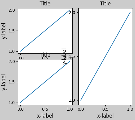
constrained_layout will not work on subplots
created via the subplot command. The reason is that each of these
commands creates a separate GridSpec instance and constrained_layout
uses (nested) gridspecs to carry out the layout. So the following fails
to yield a nice layout:
fig = plt.figure(constrained_layout=True)

ax1 = plt.subplot(221)
ax2 = plt.subplot(223)
ax3 = plt.subplot(122)

example_plot(ax1)
example_plot(ax2)
example_plot(ax3)
Of course that layout is possible using a gridspec:
fig = plt.figure(constrained_layout=True)
gs = gridspec.GridSpec(2, 2, figure=fig)

ax1 = fig.add_subplot(gs[0, 0])
ax2 = fig.add_subplot(gs[1, 0])
ax3 = fig.add_subplot(gs[:, 1])

example_plot(ax1)
example_plot(ax2)
example_plot(ax3)
Similarly,
subplot2grid() doesn’t work for the same reason:
each call creates a different parent gridspec.
fig = plt.figure(constrained_layout=True)

ax1 = plt.subplot2grid((3, 3), (0, 0))
ax2 = plt.subplot2grid((3, 3), (0, 1), colspan=2)
ax3 = plt.subplot2grid((3, 3), (1, 0), colspan=2, rowspan=2)
ax4 = plt.subplot2grid((3, 3), (1, 2), rowspan=2)

example_plot(ax1)
example_plot(ax2)
example_plot(ax3)
example_plot(ax4)
The way to make this plot compatible with constrained_layout is again
to use gridspec directly
fig = plt.figure(constrained_layout=True)
gs = gridspec.GridSpec(3, 3, figure=fig)

ax1 = fig.add_subplot(gs[0, 0])
ax2 = fig.add_subplot(gs[0, 1:])
ax3 = fig.add_subplot(gs[1:, 0:2])
ax4 = fig.add_subplot(gs[1:, -1])

example_plot(ax1)
example_plot(ax2)
example_plot(ax3)
example_plot(ax4)
constrained_layout only considers ticklabels, axis labels, titles, and
legends. Thus, other artists may be clipped and also may overlap.Constrained-layout can fail in somewhat unexpected ways. Because it uses a constraint solver the solver can find solutions that are mathematically correct, but that aren’t at all what the user wants. The usual failure mode is for all sizes to collapse to their smallest allowable value. If this happens, it is for one of two reasons:
If there is a bug, please report with a self-contained example that does not require outside data or dependencies (other than numpy).
The algorithm for the constraint is relatively straightforward, but has some complexity due to the complex ways we can layout a figure.
Figures are laid out in a hierarchy:
fig = plt.figure()
Gridspec
gs0 = gridspec.GridSpec(1, 2, figure=fig)
- Subplotspec:
ss = gs[0, 0]
- Axes:
ax0 = fig.add_subplot(ss)- Subplotspec:
ss = gs[0, 1]
Gridspec:
gsR = gridspec.GridSpecFromSubplotSpec(2, 1, ss)
Subplotspec: ss = gsR[0, 0]
- Axes:
axR0 = fig.add_subplot(ss)Subplotspec: ss = gsR[1, 0]
- Axes:
axR1 = fig.add_subplot(ss)
Each item has a layoutbox associated with it. The nesting of gridspecs
created with GridSpecFromSubplotSpec can be arbitrarily deep.
Each Axes has two layoutboxes. The first one ax._layoutbox
represents the outside of the Axes and all its decorations (i.e. ticklabels,
axis labels, etc.). The second layoutbox corresponds to the Axes’
ax.position, which sets where in the figure the spines are placed.
Why so many stacked containers? Ideally, all that would be needed are the
Axes layout boxes. For the Gridspec case, a container is
needed if the Gridspec is nested via GridSpecFromSubplotSpec. At the
top level, it is desirable for symmetry, but it also makes room for
suptitle.
For the Subplotspec/Axes case, Axes often have colorbars or other annotations that need to be packaged inside the Subplotspec, hence the need for the outer layer.
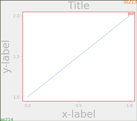
For a single Axes the layout is straight forward. The Figure and
outer Gridspec layoutboxes coincide. The Subplotspec and Axes
boxes also coincide because the Axes has no colorbar. Note
the difference between the red pos box and the green ax box
is set by the size of the decorations around the Axes.
In the code, this is accomplished by the entries in do_constrained_layout
like:
ax._poslayoutbox.edit_left_margin_min(-bbox.x0 + pos.x0 + w_padt)
from matplotlib._layoutbox import plot_children

fig, ax = plt.subplots(constrained_layout=True)
example_plot(ax, fontsize=24)
plot_children(fig, fig._layoutbox, printit=False)
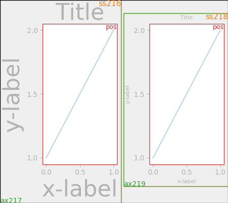
For this case, the Axes layoutboxes and the Subplotspec boxes still co-incide. However, because the decorations in the right-hand plot are so much smaller than the left-hand, so the right-hand layoutboxes are smaller.
The Subplotspec boxes are laid out in the code in the subroutine
arange_subplotspecs, which simply checks the subplotspecs in the code
against one another and stacks them appropriately.
The two pos axes are lined up. Because they have the same
minimum row, they are lined up at the top. Because
they have the same maximum row they are lined up at the bottom. In the
code this is accomplished via the calls to layoutbox.align. If
there was more than one row, then the same horizontal alignment would
occur between the rows.
The two pos axes are given the same width because the subplotspecs
occupy the same number of columns. This is accomplished in the code where
dcols0 is compared to dcolsC. If they are equal, then their widths
are constrained to be equal.
While it is a bit subtle in this case, note that the division between the Subplotspecs is not centered, but has been moved to the right to make space for the larger labels on the left-hand plot.
fig, ax = plt.subplots(1, 2, constrained_layout=True)
example_plot(ax[0], fontsize=32)
example_plot(ax[1], fontsize=8)
plot_children(fig, fig._layoutbox, printit=False)
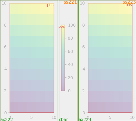
Adding a colorbar makes it clear why the Subplotspec layoutboxes must
be different from the axes layoutboxes. Here we see the left-hand
subplotspec has more room to accommodate the colorbar, and
that there are two green ax boxes inside the ss box.
Note that the width of the pos boxes is still the same because of the
constraint on their widths because their subplotspecs occupy the same
number of columns (one in this example).
The colorbar layout logic is contained in make_axes which
call _constrained_layout.layoutcolorbarsingle for cbars attached to
a single axes, and _constrained_layout.layoutcolorbargridspec if the
colorbar is associated wiht a gridspec.
fig, ax = plt.subplots(1, 2, constrained_layout=True)
im = ax[0].pcolormesh(arr, **pc_kwargs)
fig.colorbar(im, ax=ax[0], shrink=0.6)
im = ax[1].pcolormesh(arr, **pc_kwargs)
plot_children(fig, fig._layoutbox, printit=False)
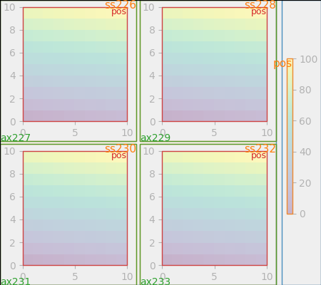
This example shows the Subplotspec layoutboxes being made smaller by
a colorbar layoutbox. The size of the colorbar layoutbox is
set to be shrink smaller than the vertical extent of the pos
layoutboxes in the gridspec, and it is made to be centered between
those two points.
fig, ax = plt.subplots(2, 2, constrained_layout=True)
for a in ax.flatten():
    im = a.pcolormesh(arr, **pc_kwargs)
fig.colorbar(im, ax=ax, shrink=0.6)
plot_children(fig, fig._layoutbox, printit=False)
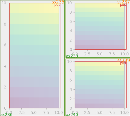
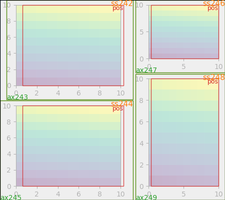
There are two ways to make axes have an uneven size in a Gridspec layout, either by specifying them to cross Gridspecs rows or columns, or by specifying width and height ratios.
The first method is used here. The constraint that makes the heights
be correct is in the code where drowsC < drows0 which in
this case would be 1 is less than 2. So we constrain the
height of the 1-row Axes to be less than half the height of the
2-row Axes.
Note
This algorithm can be wrong if the decorations attached to the smaller axes are very large, so there is an unaccounted-for edge case.
fig = plt.figure(constrained_layout=True)
gs = gridspec.GridSpec(2, 2, figure=fig)
ax = fig.add_subplot(gs[:, 0])
im = ax.pcolormesh(arr, **pc_kwargs)
ax = fig.add_subplot(gs[0, 1])
im = ax.pcolormesh(arr, **pc_kwargs)
ax = fig.add_subplot(gs[1, 1])
im = ax.pcolormesh(arr, **pc_kwargs)
plot_children(fig, fig._layoutbox, printit=False)
Height and width ratios are accommodated with the same part of the code with the smaller axes always constrained to be less in size than the larger.
fig = plt.figure(constrained_layout=True)
gs = gridspec.GridSpec(3, 2, figure=fig,
    height_ratios=[1., 0.5, 1.5],
    width_ratios=[1.2, 0.8])
ax = fig.add_subplot(gs[:2, 0])
im = ax.pcolormesh(arr, **pc_kwargs)
ax = fig.add_subplot(gs[2, 0])
im = ax.pcolormesh(arr, **pc_kwargs)
ax = fig.add_subplot(gs[0, 1])
im = ax.pcolormesh(arr, **pc_kwargs)
ax = fig.add_subplot(gs[1:, 1])
im = ax.pcolormesh(arr, **pc_kwargs)
plot_children(fig, fig._layoutbox, printit=False)
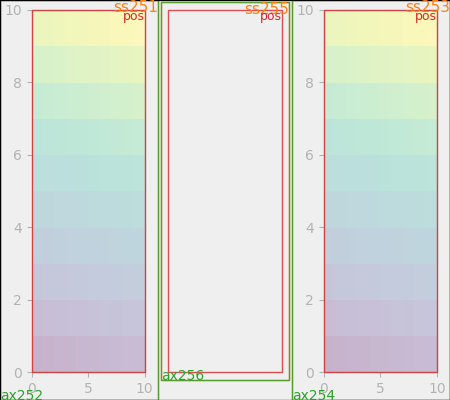
The final piece of the code that has not been explained is what happens if there is an empty gridspec opening. In that case a fake invisible axes is added and we proceed as before. The empty gridspec has no decorations, but the axes position in made the same size as the occupied Axes positions.
This is done at the start of
do_constrained_layout (hassubplotspec).
fig = plt.figure(constrained_layout=True)
gs = gridspec.GridSpec(1, 3, figure=fig)
ax = fig.add_subplot(gs[0])
im = ax.pcolormesh(arr, **pc_kwargs)
ax = fig.add_subplot(gs[-1])
im = ax.pcolormesh(arr, **pc_kwargs)
plot_children(fig, fig._layoutbox, printit=False)
plt.show()
The layout is called only once. This is OK if the original layout was pretty close (which it should be in most cases). However, if the layout changes a lot from the default layout then the decorators can change size. In particular the x and ytick labels can change. If this happens, then we should probably call the whole routine twice.
Total running time of the script: ( 0 minutes 1.904 seconds)
Keywords: matplotlib code example, codex, python plot, pyplot Gallery generated by Sphinx-Gallery