Hexbin Demo

Plotting hexbins with Matplotlib.

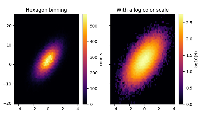
Hexbin is an axes method or pyplot function that is essentially a pcolor of a 2-D histogram with hexagonal cells. It can be much more informative than a scatter plot. In the first subplot below, try substituting ‘scatter’ for ‘hexbin’.

import numpy as np
import matplotlib.pyplot as plt
import matplotlib.mlab as mlab

# Fixing random state for reproducibility
np.random.seed(19680801)

n = 100000
x = np.random.standard_normal(n)
y = 2.0 + 3.0 * x + 4.0 * np.random.standard_normal(n)
xmin = x.min()
xmax = x.max()
ymin = y.min()
ymax = y.max()

fig, axs = plt.subplots(ncols=2, sharey=True, figsize=(7, 4))
fig.subplots_adjust(hspace=0.5, left=0.07, right=0.93)
ax = axs[0]
hb = ax.hexbin(x, y, gridsize=50, cmap='inferno')
ax.axis([xmin, xmax, ymin, ymax])
ax.set_title("Hexagon binning")
cb = fig.colorbar(hb, ax=ax)
cb.set_label('counts')

ax = axs[1]
hb = ax.hexbin(x, y, gridsize=50, bins='log', cmap='inferno')
ax.axis([xmin, xmax, ymin, ymax])
ax.set_title("With a log color scale")
cb = fig.colorbar(hb, ax=ax)
cb.set_label('log10(N)')

plt.show()

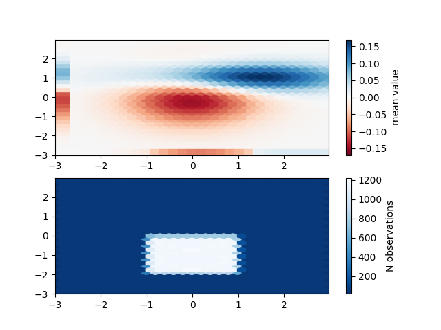
Below we’ll simulate some 2-D probability distributions, and show how to visualize them with Matplotlib.

delta = 0.025
x = y = np.arange(-3.0, 3.0, delta)
X, Y = np.meshgrid(x, y)
Z1 = mlab.bivariate_normal(X, Y, 1.0, 1.0, 0.0, 0.0)
Z2 = mlab.bivariate_normal(X, Y, 1.5, 0.5, 1, 1)
Z = Z2 - Z1  # difference of Gaussians

x = X.ravel()
y = Y.ravel()
z = Z.ravel()

# make some points 20 times more common than others, but same mean
xcond = (-1 < x) & (x < 1)
ycond = (-2 < y) & (y < 0)
cond = xcond & ycond
xnew = x[cond]
ynew = y[cond]
znew = z[cond]
for i in range(20):
    x = np.hstack((x, xnew))
    y = np.hstack((y, ynew))
    z = np.hstack((z, znew))

xmin = x.min()
xmax = x.max()
ymin = y.min()
ymax = y.max()

gridsize = 30

fig, (ax0, ax1) = plt.subplots(2, 1)

c = ax0.hexbin(x, y, C=z, gridsize=gridsize, marginals=True, cmap=plt.cm.RdBu,
               vmax=abs(z).max(), vmin=-abs(z).max())
ax0.axis([xmin, xmax, ymin, ymax])
cb = fig.colorbar(c, ax=ax0)
cb.set_label('mean value')

c = ax1.hexbin(x, y, gridsize=gridsize, cmap=plt.cm.Blues_r)
ax1.axis([xmin, xmax, ymin, ymax])
cb = fig.colorbar(c, ax=ax1)
cb.set_label('N observations')

plt.show()

Total running time of the script: ( 0 minutes 0.511 seconds)