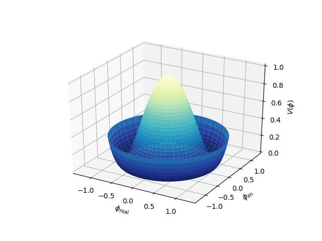
Demonstrates plotting a surface defined in polar coordinates. Uses the reversed version of the YlGnBu color map. Also demonstrates writing axis labels with latex math mode.
Example contributed by Armin Moser.
from mpl_toolkits.mplot3d import Axes3D
from matplotlib import pyplot as plt
import numpy as np


fig = plt.figure()
ax = fig.add_subplot(111, projection='3d')

# Create the mesh in polar coordinates and compute corresponding Z.
r = np.linspace(0, 1.25, 50)
p = np.linspace(0, 2*np.pi, 50)
R, P = np.meshgrid(r, p)
Z = ((R**2 - 1)**2)

# Express the mesh in the cartesian system.
X, Y = R*np.cos(P), R*np.sin(P)

# Plot the surface.
ax.plot_surface(X, Y, Z, cmap=plt.cm.YlGnBu_r)

# Tweak the limits and add latex math labels.
ax.set_zlim(0, 1)
ax.set_xlabel(r'$\phi_\mathrm{real}$')
ax.set_ylabel(r'$\phi_\mathrm{im}$')
ax.set_zlabel(r'$V(\phi)$')

plt.show()
Total running time of the script: ( 0 minutes 0.113 seconds)
