pylab_examples example code: quiver_demo.py

(Source code)

(png, pdf)

(png, pdf)

(png, pdf)

'''
========================================================
Demonstration of advanced quiver and quiverkey functions
========================================================

Known problem: the plot autoscaling does not take into account
the arrows, so those on the boundaries are often out of the picture.
This is *not* an easy problem to solve in a perfectly general way.
The workaround is to manually expand the axes.
'''
import matplotlib.pyplot as plt
import numpy as np
from numpy import ma

X, Y = np.meshgrid(np.arange(0, 2 * np.pi, .2), np.arange(0, 2 * np.pi, .2))
U = np.cos(X)
V = np.sin(Y)

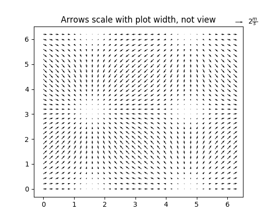
plt.figure()
plt.title('Arrows scale with plot width, not view')
Q = plt.quiver(X, Y, U, V, units='width')
qk = plt.quiverkey(Q, 0.9, 0.9, 2, r'$2 \frac{m}{s}$', labelpos='E',
                   coordinates='figure')

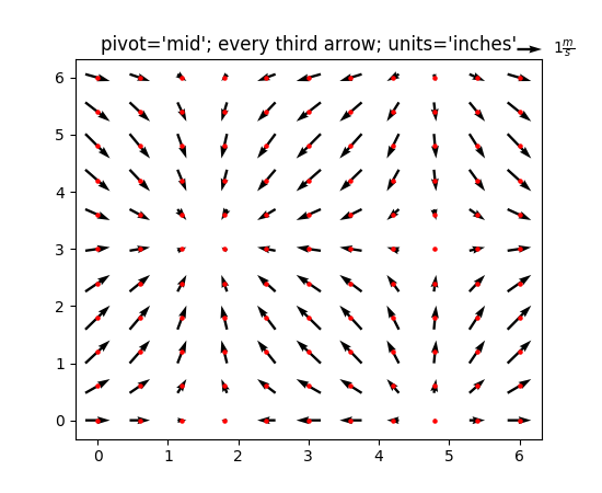
plt.figure()
plt.title("pivot='mid'; every third arrow; units='inches'")
Q = plt.quiver(X[::3, ::3], Y[::3, ::3], U[::3, ::3], V[::3, ::3],
               pivot='mid', units='inches')
qk = plt.quiverkey(Q, 0.9, 0.9, 1, r'$1 \frac{m}{s}$', labelpos='E',
                   coordinates='figure')
plt.scatter(X[::3, ::3], Y[::3, ::3], color='r', s=5)

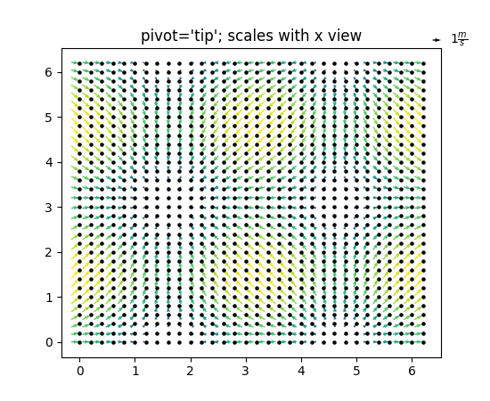
plt.figure()
plt.title("pivot='tip'; scales with x view")
M = np.hypot(U, V)
Q = plt.quiver(X, Y, U, V, M, units='x', pivot='tip', width=0.022,
               scale=1 / 0.15)
qk = plt.quiverkey(Q, 0.9, 0.9, 1, r'$1 \frac{m}{s}$', labelpos='E',
                   coordinates='figure')
plt.scatter(X, Y, color='k', s=5)

plt.show()

Keywords: python, matplotlib, pylab, example, codex (see Search examples)