

(Source code, png, pdf)

"""
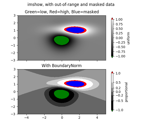
imshow with masked array input and out-of-range colors.
The second subplot illustrates the use of BoundaryNorm to
get a filled contour effect.
"""
from copy import copy
import numpy as np
import matplotlib.pyplot as plt
import matplotlib.colors as colors
import matplotlib.mlab as mlab
# compute some interesting data
x0, x1 = -5, 5
y0, y1 = -3, 3
x = np.linspace(x0, x1, 500)
y = np.linspace(y0, y1, 500)
X, Y = np.meshgrid(x, y)
Z1 = mlab.bivariate_normal(X, Y, 1.0, 1.0, 0.0, 0.0)
Z2 = mlab.bivariate_normal(X, Y, 1.5, 0.5, 1, 1)
Z = 10*(Z2 - Z1) # difference of Gaussians
# Set up a colormap:
# use copy so that we do not mutate the global colormap instance
palette = copy(plt.cm.gray)
palette.set_over('r', 1.0)
palette.set_under('g', 1.0)
palette.set_bad('b', 1.0)
# Alternatively, we could use
# palette.set_bad(alpha = 0.0)
# to make the bad region transparent. This is the default.
# If you comment out all the palette.set* lines, you will see
# all the defaults; under and over will be colored with the
# first and last colors in the palette, respectively.
Zm = np.ma.masked_where(Z > 1.2, Z)
# By setting vmin and vmax in the norm, we establish the
# range to which the regular palette color scale is applied.
# Anything above that range is colored based on palette.set_over, etc.
# set up the axes
fig, (ax1, ax2) = plt.subplots(nrows=2, figsize=(6, 5.4))
# plot using 'continuous' color map
im = ax1.imshow(Zm, interpolation='bilinear',
cmap=palette,
norm=colors.Normalize(vmin=-1.0, vmax=1.0),
aspect='auto',
origin='lower',
extent=[x0, x1, y0, y1])
ax1.set_title('Green=low, Red=high, Blue=masked')
cbar = fig.colorbar(im, extend='both', shrink=0.9, ax=ax1)
cbar.set_label('uniform')
for ticklabel in ax1.xaxis.get_ticklabels():
ticklabel.set_visible(False)
# Plot using a small number of colors, with unevenly spaced boundaries.
im = ax2.imshow(Zm, interpolation='nearest',
cmap=palette,
norm=colors.BoundaryNorm([-1, -0.5, -0.2, 0, 0.2, 0.5, 1],
ncolors=palette.N),
aspect='auto',
origin='lower',
extent=[x0, x1, y0, y1])
ax2.set_title('With BoundaryNorm')
cbar = fig.colorbar(im, extend='both', spacing='proportional',
shrink=0.9, ax=ax2)
cbar.set_label('proportional')
fig.suptitle('imshow, with out-of-range and masked data')
plt.show()
Keywords: python, matplotlib, pylab, example, codex (see Search examples)