Creating, viewing, and saving Matplotlib Figures

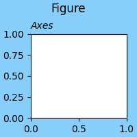
fig = plt.figure(figsize=(2, 2), facecolor='lightskyblue',
                 layout='constrained')
fig.suptitle('Figure')
ax = fig.add_subplot()
ax.set_title('Axes', loc='left', fontstyle='oblique', fontsize='medium')

(Source code, png)

When looking at Matplotlib visualization, you are almost always looking at Artists placed on a Figure. In the example above, the figure is the blue region and add_subplot has added an Axes artist to the Figure (see Parts of a Figure). A more complicated visualization can add multiple Axes to the Figure, colorbars, legends, annotations, and the Axes themselves can have multiple Artists added to them (e.g. ax.plot or ax.imshow).

Viewing Figures

We will discuss how to create Figures in more detail below, but first it is helpful to understand how to view a Figure. This varies based on how you are using Matplotlib, and what Backend you are using.

Notebooks and IDEs

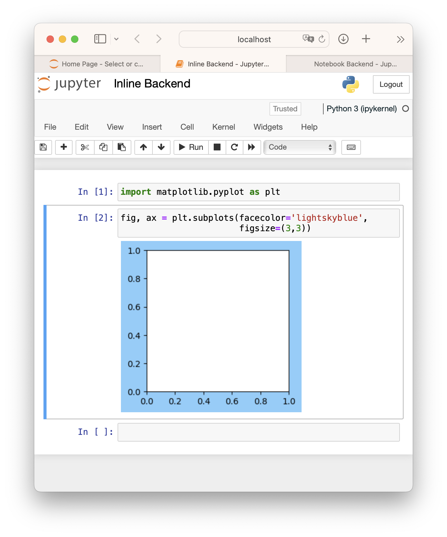
Screenshot of a Jupyter Notebook, with a figure generated via the default inline backend.

If you are using a Notebook (e.g. Jupyter) or an IDE that renders Notebooks (PyCharm, VSCode, etc), then they have a backend that will render the Matplotlib Figure when a code cell is executed. One thing to be aware of is that the default Jupyter backend (%matplotlib inline) will by default trim or expand the figure size to have a tight box around Artists added to the Figure (see Saving Figures, below). If you use a backend other than the default "inline" backend, you will likely need to use an ipython "magic" like %matplotlib notebook for the Matplotlib notebook or %matplotlib widget for the ipympl backend.

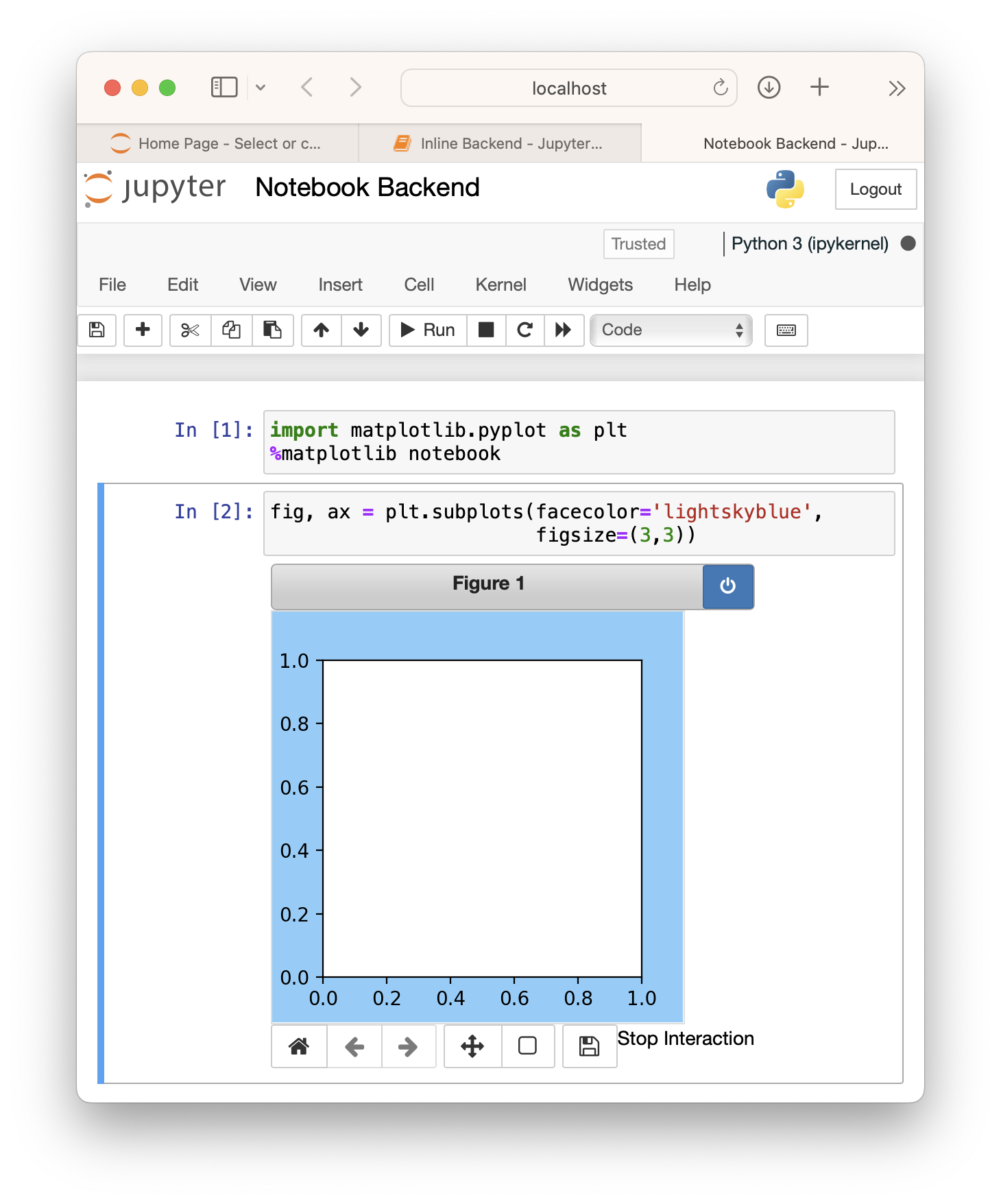
Screenshot of a Jupyter Notebook with an interactive figure generated via the %matplotlib notebook magic. Users should also try the similar widget backend if using JupyterLab.

See also

Interactive figures.

Standalone scripts and interactive use

If the user is on a client with a windowing system, there are a number of Backends that can be used to render the Figure to the screen, usually using a Python Qt, Tk, or Wx toolkit, or the native MacOS backend. These are typically chosen either in the user's matplotlibrc, or by calling, for example, matplotlib.use('QtAgg') at the beginning of a session or script.

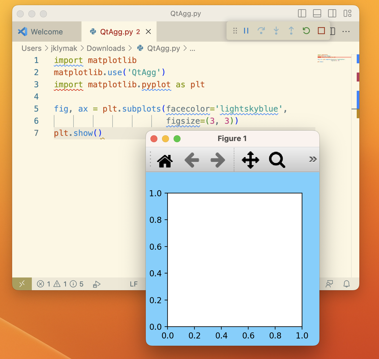
Screenshot of a Figure generated via a python script and shown using the QtAgg backend.

When run from a script, or interactively (e.g. from an iPython shell) the Figure will not be shown until we call plt.show(). The Figure will appear in a new GUI window, and usually will have a toolbar with Zoom, Pan, and other tools for interacting with the Figure. By default, plt.show() blocks further interaction from the script or shell until the Figure window is closed, though that can be toggled off for some purposes. For more details, please see Interactive mode.

Note that if you are on a client that does not have access to a windowing system, the Figure will fallback to being drawn using the "Agg" backend, and cannot be viewed, though it can be saved.

See also

Interactive figures.

Creating Figures

By far the most common way to create a figure is using the pyplot interface. As noted in Matplotlib Application Interfaces (APIs), the pyplot interface serves two purposes. One is to spin up the Backend and keep track of GUI windows. The other is a global state for Axes and Artists that allow a short-form API to plotting methods. In the example above, we use pyplot for the first purpose, and create the Figure object, fig. As a side effect fig is also added to pyplot's global state, and can be accessed via gcf.

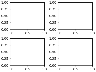
Users typically want an Axes or a grid of Axes when they create a Figure, so in addition to figure, there are convenience methods that return both a Figure and some Axes. A simple grid of Axes can be achieved with pyplot.subplots (which simply wraps Figure.subplots):

fig, axs = plt.subplots(2, 2, figsize=(4, 3), layout='constrained')

(Source code, png)

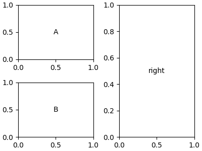
More complex grids can be achieved with pyplot.subplot_mosaic (which wraps Figure.subplot_mosaic):

fig, axs = plt.subplot_mosaic([['A', 'right'], ['B', 'right']],
                              figsize=(4, 3), layout='constrained')
for ax_name in axs:
    axs[ax_name].text(0.5, 0.5, ax_name, ha='center', va='center')

(Source code, png)

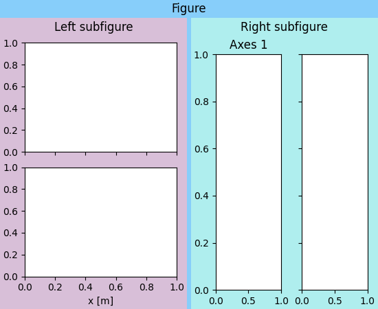
Sometimes we want to have a nested layout in a Figure, with two or more sets of Axes that do not share the same subplot grid. We can use add_subfigure or subfigures to create virtual figures inside a parent Figure; see Figure subfigures for more details.

fig = plt.figure(layout='constrained', facecolor='lightskyblue')
fig.suptitle('Figure')
figL, figR = fig.subfigures(1, 2)
figL.set_facecolor('thistle')
axL = figL.subplots(2, 1, sharex=True)
axL[1].set_xlabel('x [m]')
figL.suptitle('Left subfigure')
figR.set_facecolor('paleturquoise')
axR = figR.subplots(1, 2, sharey=True)
axR[0].set_title('Axes 1')
figR.suptitle('Right subfigure')

(Source code, png)

It is possible to directly instantiate a Figure instance without using the pyplot interface. This is usually only necessary if you want to create your own GUI application or service that you do not want carrying the pyplot global state. See the embedding examples in Embedding Matplotlib in graphical user interfaces for examples of how to do this.

Figure options

There are a few options available when creating figures. The Figure size on the screen is set by figsize and dpi. figsize is the (width, height) of the Figure in inches (or, if preferred, units of 72 typographic points). dpi are how many pixels per inch the figure will be rendered at. To make your Figures appear on the screen at the physical size you requested, you should set dpi to the same dpi as your graphics system. Note that many graphics systems now use a "dpi ratio" to specify how many screen pixels are used to represent a graphics pixel. Matplotlib applies the dpi ratio to the dpi passed to the figure to make it have higher resolution, so you should pass the lower number to the figure.

The facecolor, edgecolor, linewidth, and frameon options all change the appearance of the figure in expected ways, with frameon making the figure transparent if set to False.

Finally, the user can specify a layout engine for the figure with the layout parameter. Currently Matplotlib supplies "constrained", "compressed" and "tight" layout engines. These rescale axes inside the Figure to prevent overlap of ticklabels, and try and align axes, and can save significant manual adjustment of artists on a Figure for many common cases.

Adding Artists

The FigureBase class has a number of methods to add artists to a Figure or a SubFigure. By far the most common are to add Axes of various configurations (add_axes, add_subplot, subplots, subplot_mosaic) and subfigures (subfigures). Colorbars are added to Axes or group of Axes at the Figure level (colorbar). It is also possible to have a Figure-level legend (legend). Other Artists include figure-wide labels (suptitle, supxlabel, supylabel) and text (text). Finally, low-level Artists can be added directly using add_artist usually with care being taken to use the appropriate transform. Usually these include Figure.transFigure which ranges from 0 to 1 in each direction, and represents the fraction of the current Figure size, or Figure.dpi_scale_trans which will be in physical units of inches from the bottom left corner of the Figure (see Transformations Tutorial for more details).

Saving Figures

Finally, Figures can be saved to disk using the savefig method. fig.savefig('MyFigure.png', dpi=200) will save a PNG formatted figure to the file MyFigure.png in the current directory on disk with 200 dots-per-inch resolution. Note that the filename can include a relative or absolute path to any place on the file system.

Many types of output are supported, including raster formats like PNG, GIF, JPEG, TIFF and vector formats like PDF, EPS, and SVG.

By default, the size of the saved Figure is set by the Figure size (in inches) and, for the raster formats, the dpi. If dpi is not set, then the dpi of the Figure is used. Note that dpi still has meaning for vector formats like PDF if the Figure includes Artists that have been rasterized; the dpi specified will be the resolution of the rasterized objects.

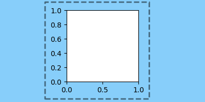
It is possible to change the size of the Figure using the bbox_inches argument to savefig. This can be specified manually, again in inches. However, by far the most common use is bbox_inches='tight'. This option "shrink-wraps", trimming or expanding as needed, the size of the figure so that it is tight around all the artists in a figure, with a small pad that can be specified by pad_inches, which defaults to 0.1 inches. The dashed box in the plot below shows the portion of the figure that would be saved if bbox_inches='tight' were used in savefig.

(Source code, png)