Note
Click here to download the full example code
Customizing Matplotlib with style sheets and rcParams
Tips for customizing the properties and default styles of Matplotlib.
Using style sheets
The style package adds support for easy-to-switch plotting
"styles" with the same parameters as a matplotlib rc file (which is read at startup to
configure Matplotlib).
There are a number of pre-defined styles provided by Matplotlib. For example, there's a pre-defined style called "ggplot", which emulates the aesthetics of ggplot (a popular plotting package for R). To use this style, just add:
import numpy as np
import matplotlib.pyplot as plt
import matplotlib as mpl
from cycler import cycler
plt.style.use('ggplot')
data = np.random.randn(50)
To list all available styles, use:
print(plt.style.available)
Out:
['Solarize_Light2', '_classic_test_patch', 'bmh', 'classic', 'dark_background', 'fast', 'fivethirtyeight', 'ggplot', 'grayscale', 'seaborn', 'seaborn-bright', 'seaborn-colorblind', 'seaborn-dark', 'seaborn-dark-palette', 'seaborn-darkgrid', 'seaborn-deep', 'seaborn-muted', 'seaborn-notebook', 'seaborn-paper', 'seaborn-pastel', 'seaborn-poster', 'seaborn-talk', 'seaborn-ticks', 'seaborn-white', 'seaborn-whitegrid', 'tableau-colorblind10']
Defining your own style
You can create custom styles and use them by calling style.use with
the path or URL to the style sheet.
For example, you might want to create
./images/presentation.mplstyle with the following:
axes.titlesize : 24
axes.labelsize : 20
lines.linewidth : 3
lines.markersize : 10
xtick.labelsize : 16
ytick.labelsize : 16
Then, when you want to adapt a plot designed for a paper to one that looks good in a presentation, you can just add:
>>> import matplotlib.pyplot as plt
>>> plt.style.use('./images/presentation.mplstyle')
Alternatively, you can make your style known to Matplotlib by placing
your <style-name>.mplstyle file into mpl_configdir/stylelib. You
can then load your custom style sheet with a call to
style.use(<style-name>). By default mpl_configdir should be
~/.config/matplotlib, but you can check where yours is with
matplotlib.get_configdir(); you may need to create this directory. You
also can change the directory where Matplotlib looks for the stylelib/
folder by setting the MPLCONFIGDIR environment variable, see
matplotlib configuration and cache directory locations.
Note that a custom style sheet in mpl_configdir/stylelib will override a
style sheet defined by Matplotlib if the styles have the same name.
Once your <style-name>.mplstyle file is in the appropriate
mpl_configdir you can specify your style with:
>>> import matplotlib.pyplot as plt
>>> plt.style.use(<style-name>)
Composing styles
Style sheets are designed to be composed together. So you can have a style sheet that customizes colors and a separate style sheet that alters element sizes for presentations. These styles can easily be combined by passing a list of styles:
>>> import matplotlib.pyplot as plt
>>> plt.style.use(['dark_background', 'presentation'])
Note that styles further to the right will overwrite values that are already defined by styles on the left.
Temporary styling
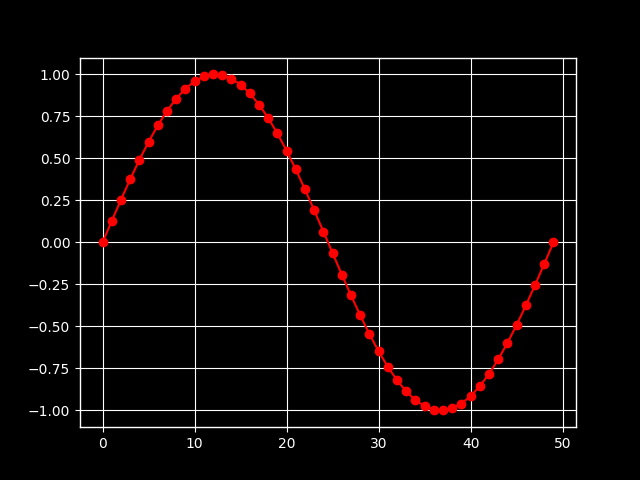
If you only want to use a style for a specific block of code but don't want to change the global styling, the style package provides a context manager for limiting your changes to a specific scope. To isolate your styling changes, you can write something like the following:
with plt.style.context('dark_background'):
    plt.plot(np.sin(np.linspace(0, 2 * np.pi)), 'r-o')
plt.show()
Matplotlib rcParams
Dynamic rc settings
You can also dynamically change the default rc settings in a python script or
interactively from the python shell. All of the rc settings are stored in a
dictionary-like variable called matplotlib.rcParams, which is global to
the matplotlib package. rcParams can be modified directly, for example:
mpl.rcParams['lines.linewidth'] = 2
mpl.rcParams['lines.linestyle'] = '--'
plt.plot(data)
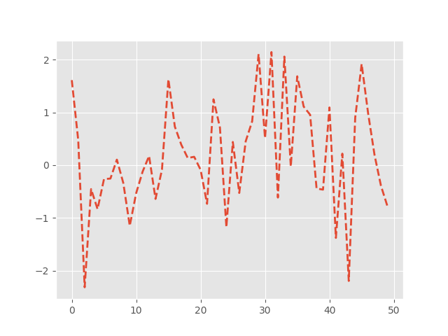
Out:
[<matplotlib.lines.Line2D object at 0x7fcbe07537f0>]
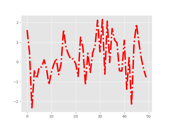
Note, that in order to change the usual plot color you have to
change the prop_cycle property of axes:
mpl.rcParams['axes.prop_cycle'] = cycler(color=['r', 'g', 'b', 'y'])
plt.plot(data)  # first color is red

Out:
[<matplotlib.lines.Line2D object at 0x7fcbe18e39a0>]
Matplotlib also provides a couple of convenience functions for modifying rc
settings. matplotlib.rc can be used to modify multiple
settings in a single group at once, using keyword arguments:
Out:
[<matplotlib.lines.Line2D object at 0x7fcbe1839250>]
matplotlib.rcdefaults will restore the standard Matplotlib
default settings.
There is some degree of validation when setting the values of rcParams, see
matplotlib.rcsetup for details.
The matplotlibrc file
Matplotlib uses matplotlibrc configuration files to customize all
kinds of properties, which we call 'rc settings' or 'rc parameters'. You can
control the defaults of almost every property in Matplotlib: figure size and
DPI, line width, color and style, axes, axis and grid properties, text and
font properties and so on. When a URL or path is not specified with a call to
style.use('<path>/<style-name>.mplstyle'), Matplotlib looks for
matplotlibrc in four locations, in the following order:
matplotlibrcin the current working directory, usually used for specific customizations that you do not want to apply elsewhere.$MATPLOTLIBRCif it is a file, else$MATPLOTLIBRC/matplotlibrc.It next looks in a user-specific place, depending on your platform:
- On Linux and FreeBSD, it looks in
.config/matplotlib/matplotlibrc(or$XDG_CONFIG_HOME/matplotlib/matplotlibrc) if you've customized your environment. - On other platforms, it looks in
.matplotlib/matplotlibrc.
- On Linux and FreeBSD, it looks in
INSTALL/matplotlib/mpl-data/matplotlibrc, whereINSTALLis something like/usr/lib/python3.7/site-packageson Linux, and maybeC:\Python37\Lib\site-packageson Windows. Every time you install matplotlib, this file will be overwritten, so if you want your customizations to be saved, please move this file to your user-specific matplotlib directory.
Once a matplotlibrc file has been found, it will not search any of
the other paths.
To display where the currently active matplotlibrc file was
loaded from, one can do the following:
>>> import matplotlib
>>> matplotlib.matplotlib_fname()
'/home/foo/.config/matplotlib/matplotlibrc'
See below for a sample matplotlibrc file.
A sample matplotlibrc file
#### MATPLOTLIBRC FORMAT
## NOTE FOR END USERS: DO NOT EDIT THIS FILE!
##
## This is a sample matplotlib configuration file - you can find a copy
## of it on your system in site-packages/matplotlib/mpl-data/matplotlibrc
## (which related to your Python installation location).
##
## You should find a copy of it on your system at
## site-packages/matplotlib/mpl-data/matplotlibrc (relative to your Python
## installation location). DO NOT EDIT IT!
##
## If you wish to change your default style, copy this file to one of the
## following locations
## unix/linux:
## $HOME/.config/matplotlib/matplotlibrc OR
## $XDG_CONFIG_HOME/matplotlib/matplotlibrc (if $XDG_CONFIG_HOME is set)
## other platforms:
## $HOME/.matplotlib/matplotlibrc
## and edit that copy.
##
## See https://matplotlib.org/users/customizing.html#the-matplotlibrc-file
## for more details on the paths which are checked for the configuration file.
##
## Blank lines, or lines starting with a comment symbol, are ignored, as are
## trailing comments. Other lines must have the format:
## key: val # optional comment
##
## Formatting: Use PEP8-like style (as enforced in the rest of the codebase).
## All lines start with an additional '#', so that removing all leading '#'s
## yields a valid style file.
##
## Colors: for the color values below, you can either use
## - a matplotlib color string, such as r, k, or b
## - an rgb tuple, such as (1.0, 0.5, 0.0)
## - a hex string, such as ff00ff
## - a scalar grayscale intensity such as 0.75
## - a legal html color name, e.g., red, blue, darkslategray
##
## Matplotlib configuration are currently divided into following parts:
## - BACKENDS
## - LINES
## - PATCHES
## - HATCHES
## - BOXPLOT
## - FONT
## - TEXT
## - LaTeX
## - AXES
## - DATES
## - TICKS
## - GRIDS
## - LEGEND
## - FIGURE
## - IMAGES
## - CONTOUR PLOTS
## - ERRORBAR PLOTS
## - HISTOGRAM PLOTS
## - SCATTER PLOTS
## - AGG RENDERING
## - PATHS
## - SAVING FIGURES
## - INTERACTIVE KEYMAPS
## - ANIMATION
##### CONFIGURATION BEGINS HERE
## ***************************************************************************
## * BACKENDS *
## ***************************************************************************
## The default backend. If you omit this parameter, the first working
## backend from the following list is used:
## MacOSX Qt5Agg Gtk3Agg TkAgg WxAgg Agg
## Other choices include:
## Qt5Cairo GTK3Cairo TkCairo WxCairo Cairo
## Qt4Agg Qt4Cairo Wx # deprecated.
## PS PDF SVG Template
## You can also deploy your own backend outside of matplotlib by referring to
## the module name (which must be in the PYTHONPATH) as 'module://my_backend'.
#backend: Agg
## The port to use for the web server in the WebAgg backend.
#webagg.port: 8988
## The address on which the WebAgg web server should be reachable
#webagg.address: 127.0.0.1
## If webagg.port is unavailable, a number of other random ports will
## be tried until one that is available is found.
#webagg.port_retries: 50
## When True, open the webbrowser to the plot that is shown
#webagg.open_in_browser: True
## If you are running pyplot inside a GUI and your backend choice
## conflicts, we will automatically try to find a compatible one for
## you if backend_fallback is True
#backend_fallback: True
#interactive: False
#toolbar: toolbar2 # {None, toolbar2, toolmanager}
#timezone: UTC # a pytz timezone string, e.g., US/Central or Europe/Paris
## ***************************************************************************
## * LINES *
## ***************************************************************************
## See https://matplotlib.org/api/artist_api.html#module-matplotlib.lines
## for more information on line properties.
#lines.linewidth: 1.5 # line width in points
#lines.linestyle: - # solid line
#lines.color: C0 # has no affect on plot(); see axes.prop_cycle
#lines.marker: None # the default marker
#lines.markerfacecolor: auto # the default marker face color
#lines.markeredgecolor: auto # the default marker edge color
#lines.markeredgewidth: 1.0 # the line width around the marker symbol
#lines.markersize: 6 # marker size, in points
#lines.dash_joinstyle: round # {miter, round, bevel}
#lines.dash_capstyle: butt # {butt, round, projecting}
#lines.solid_joinstyle: round # {miter, round, bevel}
#lines.solid_capstyle: projecting # {butt, round, projecting}
#lines.antialiased: True # render lines in antialiased (no jaggies)
## The three standard dash patterns. These are scaled by the linewidth.
#lines.dashed_pattern: 3.7, 1.6
#lines.dashdot_pattern: 6.4, 1.6, 1, 1.6
#lines.dotted_pattern: 1, 1.65
#lines.scale_dashes: True
#markers.fillstyle: full # {full, left, right, bottom, top, none}
#pcolor.shading : flat
## ***************************************************************************
## * PATCHES *
## ***************************************************************************
## Patches are graphical objects that fill 2D space, like polygons or circles.
## See https://matplotlib.org/api/artist_api.html#module-matplotlib.patches
## for more information on patch properties.
#patch.linewidth: 1 # edge width in points.
#patch.facecolor: C0
#patch.edgecolor: black # if forced, or patch is not filled
#patch.force_edgecolor: False # True to always use edgecolor
#patch.antialiased: True # render patches in antialiased (no jaggies)
## ***************************************************************************
## * HATCHES *
## ***************************************************************************
#hatch.color: black
#hatch.linewidth: 1.0
## ***************************************************************************
## * BOXPLOT *
## ***************************************************************************
#boxplot.notch: False
#boxplot.vertical: True
#boxplot.whiskers: 1.5
#boxplot.bootstrap: None
#boxplot.patchartist: False
#boxplot.showmeans: False
#boxplot.showcaps: True
#boxplot.showbox: True
#boxplot.showfliers: True
#boxplot.meanline: False
#boxplot.flierprops.color: black
#boxplot.flierprops.marker: o
#boxplot.flierprops.markerfacecolor: none
#boxplot.flierprops.markeredgecolor: black
#boxplot.flierprops.markeredgewidth: 1.0
#boxplot.flierprops.markersize: 6
#boxplot.flierprops.linestyle: none
#boxplot.flierprops.linewidth: 1.0
#boxplot.boxprops.color: black
#boxplot.boxprops.linewidth: 1.0
#boxplot.boxprops.linestyle: -
#boxplot.whiskerprops.color: black
#boxplot.whiskerprops.linewidth: 1.0
#boxplot.whiskerprops.linestyle: -
#boxplot.capprops.color: black
#boxplot.capprops.linewidth: 1.0
#boxplot.capprops.linestyle: -
#boxplot.medianprops.color: C1
#boxplot.medianprops.linewidth: 1.0
#boxplot.medianprops.linestyle: -
#boxplot.meanprops.color: C2
#boxplot.meanprops.marker: ^
#boxplot.meanprops.markerfacecolor: C2
#boxplot.meanprops.markeredgecolor: C2
#boxplot.meanprops.markersize: 6
#boxplot.meanprops.linestyle: --
#boxplot.meanprops.linewidth: 1.0
## ***************************************************************************
## * FONT *
## ***************************************************************************
## The font properties used by `text.Text`.
## See https://matplotlib.org/api/font_manager_api.html for more information
## on font properties. The 6 font properties used for font matching are
## given below with their default values.
##
## The font.family property has five values:
## - 'serif' (e.g., Times),
## - 'sans-serif' (e.g., Helvetica),
## - 'cursive' (e.g., Zapf-Chancery),
## - 'fantasy' (e.g., Western), and
## - 'monospace' (e.g., Courier).
## Each of these font families has a default list of font names in decreasing
## order of priority associated with them. When text.usetex is False,
## font.family may also be one or more concrete font names.
##
## The font.style property has three values: normal (or roman), italic
## or oblique. The oblique style will be used for italic, if it is not
## present.
##
## The font.variant property has two values: normal or small-caps. For
## TrueType fonts, which are scalable fonts, small-caps is equivalent
## to using a font size of 'smaller', or about 83%% of the current font
## size.
##
## The font.weight property has effectively 13 values: normal, bold,
## bolder, lighter, 100, 200, 300, ..., 900. Normal is the same as
## 400, and bold is 700. bolder and lighter are relative values with
## respect to the current weight.
##
## The font.stretch property has 11 values: ultra-condensed,
## extra-condensed, condensed, semi-condensed, normal, semi-expanded,
## expanded, extra-expanded, ultra-expanded, wider, and narrower. This
## property is not currently implemented.
##
## The font.size property is the default font size for text, given in pts.
## 10 pt is the standard value.
##
## Note that font.size controls default text sizes. To configure
## special text sizes tick labels, axes, labels, title, etc, see the rc
## settings for axes and ticks. Special text sizes can be defined
## relative to font.size, using the following values: xx-small, x-small,
## small, medium, large, x-large, xx-large, larger, or smaller
#font.family: sans-serif
#font.style: normal
#font.variant: normal
#font.weight: normal
#font.stretch: normal
#font.size: 10.0
#font.serif: DejaVu Serif, Bitstream Vera Serif, Computer Modern Roman, New Century Schoolbook, Century Schoolbook L, Utopia, ITC Bookman, Bookman, Nimbus Roman No9 L, Times New Roman, Times, Palatino, Charter, serif
#font.sans-serif: DejaVu Sans, Bitstream Vera Sans, Computer Modern Sans Serif, Lucida Grande, Verdana, Geneva, Lucid, Arial, Helvetica, Avant Garde, sans-serif
#font.cursive: Apple Chancery, Textile, Zapf Chancery, Sand, Script MT, Felipa, cursive
#font.fantasy: Comic Neue, Comic Sans MS, Chicago, Charcoal, ImpactWestern, Humor Sans, xkcd, fantasy
#font.monospace: DejaVu Sans Mono, Bitstream Vera Sans Mono, Computer Modern Typewriter, Andale Mono, Nimbus Mono L, Courier New, Courier, Fixed, Terminal, monospace
## ***************************************************************************
## * TEXT *
## ***************************************************************************
## The text properties used by `text.Text`.
## See https://matplotlib.org/api/artist_api.html#module-matplotlib.text
## for more information on text properties
#text.color: black
## ***************************************************************************
## * LaTeX *
## ***************************************************************************
## For more information on LaTex properties, see
## https://matplotlib.org/tutorials/text/usetex.html
#text.usetex: False # use latex for all text handling. The following fonts
# are supported through the usual rc parameter settings:
# new century schoolbook, bookman, times, palatino,
# zapf chancery, charter, serif, sans-serif, helvetica,
# avant garde, courier, monospace, computer modern roman,
# computer modern sans serif, computer modern typewriter
# If another font is desired which can loaded using the
# LaTeX \usepackage command, please inquire at the
# matplotlib mailing list
#text.latex.preamble: # IMPROPER USE OF THIS FEATURE WILL LEAD TO LATEX FAILURES
# AND IS THEREFORE UNSUPPORTED. PLEASE DO NOT ASK FOR HELP
# IF THIS FEATURE DOES NOT DO WHAT YOU EXPECT IT TO.
# text.latex.preamble is a single line of LaTeX code that
# will be passed on to the LaTeX system. It may contain
# any code that is valid for the LaTeX "preamble", i.e.
# between the "\documentclass" and "\begin{document}"
# statements.
# Note that it has to be put on a single line, which may
# become quite long.
# The following packages are always loaded with usetex, so
# beware of package collisions: color, geometry, graphicx,
# type1cm, textcomp.
# Adobe Postscript (PSSNFS) font packages may also be
# loaded, depending on your font settings.
## FreeType hinting flag ("foo" corresponds to FT_LOAD_FOO); may be one of the
## following (Proprietary Matplotlib-specific synonyms are given in parentheses,
## but their use is discouraged):
## - default: Use the font's native hinter if possible, else FreeType's auto-hinter.
## ("either" is a synonym).
## - no_autohint: Use the font's native hinter if possible, else don't hint.
## ("native" is a synonym.)
## - force_autohint: Use FreeType's auto-hinter. ("auto" is a synonym.)
## - no_hinting: Disable hinting. ("none" is a synonym.)
#text.hinting: force_autohint
#text.hinting_factor: 8 # Specifies the amount of softness for hinting in the
# horizontal direction. A value of 1 will hint to full
# pixels. A value of 2 will hint to half pixels etc.
#text.kerning_factor : 0 # Specifies the scaling factor for kerning values. This
# is provided solely to allow old test images to remain
# unchanged. Set to 6 to obtain previous behavior. Values
# other than 0 or 6 have no defined meaning.
#text.antialiased: True # If True (default), the text will be antialiased.
# This only affects the Agg backend.
## The following settings allow you to select the fonts in math mode.
#mathtext.fontset: dejavusans # Should be 'dejavusans' (default),
# 'dejavuserif', 'cm' (Computer Modern), 'stix',
# 'stixsans' or 'custom' (unsupported, may go
# away in the future)
## "mathtext.fontset: custom" is defined by the mathtext.bf, .cal, .it, ...
## settings which map a TeX font name to a fontconfig font pattern. (These
## settings are not used for other font sets.)
#mathtext.bf: sans:bold
#mathtext.cal: cursive
#mathtext.it: sans:italic
#mathtext.rm: sans
#mathtext.sf: sans
#mathtext.tt: monospace
#mathtext.fallback: cm # Select fallback font from ['cm' (Computer Modern), 'stix'
# 'stixsans'] when a symbol can not be found in one of the
# custom math fonts. Select 'None' to not perform fallback
# and replace the missing character by a dummy symbol.
#mathtext.default: it # The default font to use for math.
# Can be any of the LaTeX font names, including
# the special name "regular" for the same font
# used in regular text.
## ***************************************************************************
## * AXES *
## ***************************************************************************
## Following are default face and edge colors, default tick sizes,
## default fontsizes for ticklabels, and so on. See
## https://matplotlib.org/api/axes_api.html#module-matplotlib.axes
#axes.facecolor: white # axes background color
#axes.edgecolor: black # axes edge color
#axes.linewidth: 0.8 # edge linewidth
#axes.grid: False # display grid or not
#axes.grid.axis: both # which axis the grid should apply to
#axes.grid.which: major # gridlines at {major, minor, both} ticks
#axes.titlelocation: center # alignment of the title: {left, right, center}
#axes.titlesize: large # fontsize of the axes title
#axes.titleweight: normal # font weight of title
#axes.titlecolor: auto # color of the axes title, auto falls back to
# text.color as default value
#axes.titley: None # position title (axes relative units). None implies auto
#axes.titlepad: 6.0 # pad between axes and title in points
#axes.labelsize: medium # fontsize of the x any y labels
#axes.labelpad: 4.0 # space between label and axis
#axes.labelweight: normal # weight of the x and y labels
#axes.labelcolor: black
#axes.axisbelow: line # draw axis gridlines and ticks:
# - below patches (True)
# - above patches but below lines ('line')
# - above all (False)
#axes.formatter.limits: -5, 6 # use scientific notation if log10
# of the axis range is smaller than the
# first or larger than the second
#axes.formatter.use_locale: False # When True, format tick labels
# according to the user's locale.
# For example, use ',' as a decimal
# separator in the fr_FR locale.
#axes.formatter.use_mathtext: False # When True, use mathtext for scientific
# notation.
#axes.formatter.min_exponent: 0 # minimum exponent to format in scientific notation
#axes.formatter.useoffset: True # If True, the tick label formatter
# will default to labeling ticks relative
# to an offset when the data range is
# small compared to the minimum absolute
# value of the data.
#axes.formatter.offset_threshold: 4 # When useoffset is True, the offset
# will be used when it can remove
# at least this number of significant
# digits from tick labels.
#axes.spines.left: True # display axis spines
#axes.spines.bottom: True
#axes.spines.top: True
#axes.spines.right: True
#axes.unicode_minus: True # use Unicode for the minus symbol rather than hyphen. See
# https://en.wikipedia.org/wiki/Plus_and_minus_signs#Character_codes
#axes.prop_cycle: cycler('color', ['1f77b4', 'ff7f0e', '2ca02c', 'd62728', '9467bd', '8c564b', 'e377c2', '7f7f7f', 'bcbd22', '17becf'])
# color cycle for plot lines as list of string colorspecs:
# single letter, long name, or web-style hex
# As opposed to all other paramters in this file, the color
# values must be enclosed in quotes for this parameter,
# e.g. '1f77b4', instead of 1f77b4.
# See also https://matplotlib.org/tutorials/intermediate/color_cycle.html
# for more details on prop_cycle usage.
#axes.autolimit_mode: data # How to scale axes limits to the data. By using:
# - "data" to use data limits, plus some margin
# - "round_numbers" move to the nearest "round" number
#axes.xmargin: .05 # x margin. See `axes.Axes.margins`
#axes.ymargin: .05 # y margin. See `axes.Axes.margins`
#polaraxes.grid: True # display grid on polar axes
#axes3d.grid: True # display grid on 3d axes
## ***************************************************************************
## * AXIS *
## ***************************************************************************
#xaxis.labellocation: center # alignment of the xaxis label: {left, right, center}
#yaxis.labellocation: center # alignment of the yaxis label: {bottom, top, center}
## ***************************************************************************
## * DATES *
## ***************************************************************************
## These control the default format strings used in AutoDateFormatter.
## Any valid format datetime format string can be used (see the python
## `datetime` for details). For example, by using:
## - '%%x' will use the locale date representation
## - '%%X' will use the locale time representation
## - '%%c' will use the full locale datetime representation
## These values map to the scales:
## {'year': 365, 'month': 30, 'day': 1, 'hour': 1/24, 'minute': 1 / (24 * 60)}
#date.autoformatter.year: %Y
#date.autoformatter.month: %Y-%m
#date.autoformatter.day: %Y-%m-%d
#date.autoformatter.hour: %m-%d %H
#date.autoformatter.minute: %d %H:%M
#date.autoformatter.second: %H:%M:%S
#date.autoformatter.microsecond: %M:%S.%f
## The reference date for Matplotlib's internal date representation
## See https://matplotlib.org/examples/ticks_and_spines/date_precision_and_epochs.py
#date.epoch: 1970-01-01T00:00:00
## ***************************************************************************
## * TICKS *
## ***************************************************************************
## See https://matplotlib.org/api/axis_api.html#matplotlib.axis.Tick
#xtick.top: False # draw ticks on the top side
#xtick.bottom: True # draw ticks on the bottom side
#xtick.labeltop: False # draw label on the top
#xtick.labelbottom: True # draw label on the bottom
#xtick.major.size: 3.5 # major tick size in points
#xtick.minor.size: 2 # minor tick size in points
#xtick.major.width: 0.8 # major tick width in points
#xtick.minor.width: 0.6 # minor tick width in points
#xtick.major.pad: 3.5 # distance to major tick label in points
#xtick.minor.pad: 3.4 # distance to the minor tick label in points
#xtick.color: black # color of the tick labels
#xtick.labelsize: medium # fontsize of the tick labels
#xtick.direction: out # direction: {in, out, inout}
#xtick.minor.visible: False # visibility of minor ticks on x-axis
#xtick.major.top: True # draw x axis top major ticks
#xtick.major.bottom: True # draw x axis bottom major ticks
#xtick.minor.top: True # draw x axis top minor ticks
#xtick.minor.bottom: True # draw x axis bottom minor ticks
#xtick.alignment: center # alignment of xticks
#ytick.left: True # draw ticks on the left side
#ytick.right: False # draw ticks on the right side
#ytick.labelleft: True # draw tick labels on the left side
#ytick.labelright: False # draw tick labels on the right side
#ytick.major.size: 3.5 # major tick size in points
#ytick.minor.size: 2 # minor tick size in points
#ytick.major.width: 0.8 # major tick width in points
#ytick.minor.width: 0.6 # minor tick width in points
#ytick.major.pad: 3.5 # distance to major tick label in points
#ytick.minor.pad: 3.4 # distance to the minor tick label in points
#ytick.color: black # color of the tick labels
#ytick.labelsize: medium # fontsize of the tick labels
#ytick.direction: out # direction: {in, out, inout}
#ytick.minor.visible: False # visibility of minor ticks on y-axis
#ytick.major.left: True # draw y axis left major ticks
#ytick.major.right: True # draw y axis right major ticks
#ytick.minor.left: True # draw y axis left minor ticks
#ytick.minor.right: True # draw y axis right minor ticks
#ytick.alignment: center_baseline # alignment of yticks
## ***************************************************************************
## * GRIDS *
## ***************************************************************************
#grid.color: b0b0b0 # grid color
#grid.linestyle: - # solid
#grid.linewidth: 0.8 # in points
#grid.alpha: 1.0 # transparency, between 0.0 and 1.0
## ***************************************************************************
## * LEGEND *
## ***************************************************************************
#legend.loc: best
#legend.frameon: True # if True, draw the legend on a background patch
#legend.framealpha: 0.8 # legend patch transparency
#legend.facecolor: inherit # inherit from axes.facecolor; or color spec
#legend.edgecolor: 0.8 # background patch boundary color
#legend.fancybox: True # if True, use a rounded box for the
# legend background, else a rectangle
#legend.shadow: False # if True, give background a shadow effect
#legend.numpoints: 1 # the number of marker points in the legend line
#legend.scatterpoints: 1 # number of scatter points
#legend.markerscale: 1.0 # the relative size of legend markers vs. original
#legend.fontsize: medium
#legend.title_fontsize: None # None sets to the same as the default axes.
## Dimensions as fraction of fontsize:
#legend.borderpad: 0.4 # border whitespace
#legend.labelspacing: 0.5 # the vertical space between the legend entries
#legend.handlelength: 2.0 # the length of the legend lines
#legend.handleheight: 0.7 # the height of the legend handle
#legend.handletextpad: 0.8 # the space between the legend line and legend text
#legend.borderaxespad: 0.5 # the border between the axes and legend edge
#legend.columnspacing: 2.0 # column separation
## ***************************************************************************
## * FIGURE *
## ***************************************************************************
## See https://matplotlib.org/api/figure_api.html#matplotlib.figure.Figure
#figure.titlesize: large # size of the figure title (``Figure.suptitle()``)
#figure.titleweight: normal # weight of the figure title
#figure.figsize: 6.4, 4.8 # figure size in inches
#figure.dpi: 100 # figure dots per inch
#figure.facecolor: white # figure facecolor
#figure.edgecolor: white # figure edgecolor
#figure.frameon: True # enable figure frame
#figure.max_open_warning: 20 # The maximum number of figures to open through
# the pyplot interface before emitting a warning.
# If less than one this feature is disabled.
#figure.raise_window : True # Raise the GUI window to front when show() is called.
## The figure subplot parameters. All dimensions are a fraction of the figure width and height.
#figure.subplot.left: 0.125 # the left side of the subplots of the figure
#figure.subplot.right: 0.9 # the right side of the subplots of the figure
#figure.subplot.bottom: 0.11 # the bottom of the subplots of the figure
#figure.subplot.top: 0.88 # the top of the subplots of the figure
#figure.subplot.wspace: 0.2 # the amount of width reserved for space between subplots,
# expressed as a fraction of the average axis width
#figure.subplot.hspace: 0.2 # the amount of height reserved for space between subplots,
# expressed as a fraction of the average axis height
## Figure layout
#figure.autolayout: False # When True, automatically adjust subplot
# parameters to make the plot fit the figure
# using `tight_layout`
#figure.constrained_layout.use: False # When True, automatically make plot
# elements fit on the figure. (Not
# compatible with `autolayout`, above).
#figure.constrained_layout.h_pad: 0.04167 # Padding around axes objects. Float representing
#figure.constrained_layout.w_pad: 0.04167 # inches. Default is 3./72. inches (3 pts)
#figure.constrained_layout.hspace: 0.02 # Space between subplot groups. Float representing
#figure.constrained_layout.wspace: 0.02 # a fraction of the subplot widths being separated.
## ***************************************************************************
## * IMAGES *
## ***************************************************************************
#image.aspect: equal # {equal, auto} or a number
#image.interpolation: antialiased # see help(imshow) for options
#image.cmap: viridis # A colormap name, gray etc...
#image.lut: 256 # the size of the colormap lookup table
#image.origin: upper # {lower, upper}
#image.resample: True
#image.composite_image: True # When True, all the images on a set of axes are
# combined into a single composite image before
# saving a figure as a vector graphics file,
# such as a PDF.
## ***************************************************************************
## * CONTOUR PLOTS *
## ***************************************************************************
#contour.negative_linestyle: dashed # string or on-off ink sequence
#contour.corner_mask: True # {True, False, legacy}
#contour.linewidth: None # {float, None} Size of the contour
# linewidths. If set to None,
# it falls back to `line.linewidth`.
## ***************************************************************************
## * ERRORBAR PLOTS *
## ***************************************************************************
#errorbar.capsize: 0 # length of end cap on error bars in pixels
## ***************************************************************************
## * HISTOGRAM PLOTS *
## ***************************************************************************
#hist.bins: 10 # The default number of histogram bins or 'auto'.
## ***************************************************************************
## * SCATTER PLOTS *
## ***************************************************************************
#scatter.marker: o # The default marker type for scatter plots.
#scatter.edgecolors: face # The default edge colors for scatter plots.
## ***************************************************************************
## * AGG RENDERING *
## ***************************************************************************
## Warning: experimental, 2008/10/10
#agg.path.chunksize: 0 # 0 to disable; values in the range
# 10000 to 100000 can improve speed slightly
# and prevent an Agg rendering failure
# when plotting very large data sets,
# especially if they are very gappy.
# It may cause minor artifacts, though.
# A value of 20000 is probably a good
# starting point.
## ***************************************************************************
## * PATHS *
## ***************************************************************************
#path.simplify: True # When True, simplify paths by removing "invisible"
# points to reduce file size and increase rendering
# speed
#path.simplify_threshold: 0.111111111111 # The threshold of similarity below
# which vertices will be removed in
# the simplification process.
#path.snap: True # When True, rectilinear axis-aligned paths will be snapped
# to the nearest pixel when certain criteria are met.
# When False, paths will never be snapped.
#path.sketch: None # May be None, or a 3-tuple of the form:
# (scale, length, randomness).
# - *scale* is the amplitude of the wiggle
# perpendicular to the line (in pixels).
# - *length* is the length of the wiggle along the
# line (in pixels).
# - *randomness* is the factor by which the length is
# randomly scaled.
#path.effects:
## ***************************************************************************
## * SAVING FIGURES *
## ***************************************************************************
## The default savefig params can be different from the display params
## e.g., you may want a higher resolution, or to make the figure
## background white
#savefig.dpi: figure # figure dots per inch or 'figure'
#savefig.facecolor: auto # figure facecolor when saving
#savefig.edgecolor: auto # figure edgecolor when saving
#savefig.format: png # {png, ps, pdf, svg}
#savefig.bbox: standard # {tight, standard}
# 'tight' is incompatible with pipe-based animation
# backends (e.g. 'ffmpeg') but will work with those
# based on temporary files (e.g. 'ffmpeg_file')
#savefig.pad_inches: 0.1 # Padding to be used when bbox is set to 'tight'
#savefig.directory: ~ # default directory in savefig dialog box,
# leave empty to always use current working directory
#savefig.transparent: False # setting that controls whether figures are saved with a
# transparent background by default
#savefig.orientation: portrait # Orientation of saved figure
### tk backend params
#tk.window_focus: False # Maintain shell focus for TkAgg
### ps backend params
#ps.papersize: letter # {auto, letter, legal, ledger, A0-A10, B0-B10}
#ps.useafm: False # use of afm fonts, results in small files
#ps.usedistiller: False # {ghostscript, xpdf, None}
# Experimental: may produce smaller files.
# xpdf intended for production of publication quality files,
# but requires ghostscript, xpdf and ps2eps
#ps.distiller.res: 6000 # dpi
#ps.fonttype: 3 # Output Type 3 (Type3) or Type 42 (TrueType)
### PDF backend params
#pdf.compression: 6 # integer from 0 to 9
# 0 disables compression (good for debugging)
#pdf.fonttype: 3 # Output Type 3 (Type3) or Type 42 (TrueType)
#pdf.use14corefonts : False
#pdf.inheritcolor: False
### SVG backend params
#svg.image_inline: True # Write raster image data directly into the SVG file
#svg.fonttype: path # How to handle SVG fonts:
# path: Embed characters as paths -- supported
# by most SVG renderers
# None: Assume fonts are installed on the
# machine where the SVG will be viewed.
#svg.hashsalt: None # If not None, use this string as hash salt instead of uuid4
### pgf parameter
## See https://matplotlib.org/tutorials/text/pgf.html for more information.
#pgf.rcfonts: True
#pgf.preamble: # See text.latex.preamble for documentation
#pgf.texsystem: xelatex
### docstring params
#docstring.hardcopy: False # set this when you want to generate hardcopy docstring
## ***************************************************************************
## * INTERACTIVE KEYMAPS *
## ***************************************************************************
## Event keys to interact with figures/plots via keyboard.
## See https://matplotlib.org/users/navigation_toolbar.html for more details on
## interactive navigation. Customize these settings according to your needs.
## Leave the field(s) empty if you don't need a key-map. (i.e., fullscreen : '')
#keymap.fullscreen: f, ctrl+f # toggling
#keymap.home: h, r, home # home or reset mnemonic
#keymap.back: left, c, backspace, MouseButton.BACK # forward / backward keys
#keymap.forward: right, v, MouseButton.FORWARD # for quick navigation
#keymap.pan: p # pan mnemonic
#keymap.zoom: o # zoom mnemonic
#keymap.save: s, ctrl+s # saving current figure
#keymap.help: f1 # display help about active tools
#keymap.quit: ctrl+w, cmd+w, q # close the current figure
#keymap.quit_all: # close all figures
#keymap.grid: g # switching on/off major grids in current axes
#keymap.grid_minor: G # switching on/off minor grids in current axes
#keymap.yscale: l # toggle scaling of y-axes ('log'/'linear')
#keymap.xscale: k, L # toggle scaling of x-axes ('log'/'linear')
#keymap.copy: ctrl+c, cmd+c # Copy figure to clipboard
## ***************************************************************************
## * ANIMATION *
## ***************************************************************************
#animation.html: none # How to display the animation as HTML in
# the IPython notebook:
# - 'html5' uses HTML5 video tag
# - 'jshtml' creates a Javascript animation
#animation.writer: ffmpeg # MovieWriter 'backend' to use
#animation.codec: h264 # Codec to use for writing movie
#animation.bitrate: -1 # Controls size/quality tradeoff for movie.
# -1 implies let utility auto-determine
#animation.frame_format: png # Controls frame format used by temp files
#animation.ffmpeg_path: ffmpeg # Path to ffmpeg binary. Without full path
# $PATH is searched
#animation.ffmpeg_args: # Additional arguments to pass to ffmpeg
#animation.convert_path: convert # Path to ImageMagick's convert binary.
# On Windows use the full path since convert
# is also the name of a system tool.
#animation.convert_args: # Additional arguments to pass to convert
#animation.embed_limit: 20.0 # Limit, in MB, of size of base64 encoded
# animation in HTML (i.e. IPython notebook)
#mpl_toolkits.legacy_colorbar: True
Total running time of the script: ( 0 minutes 1.561 seconds)
Keywords: matplotlib code example, codex, python plot, pyplot Gallery generated by Sphinx-Gallery