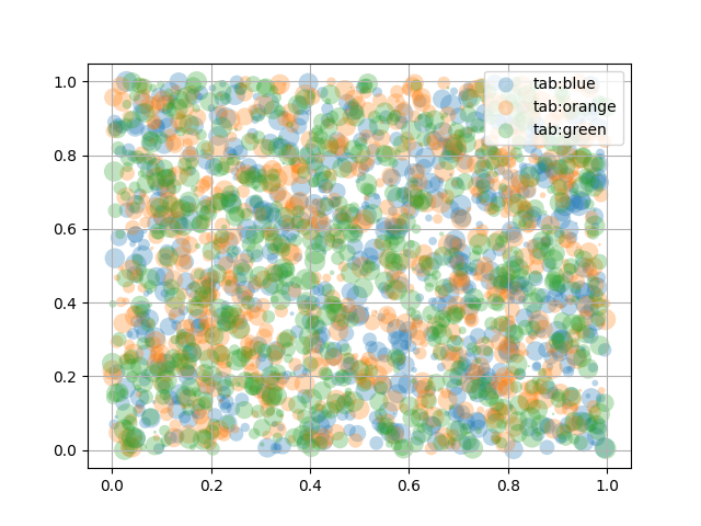
Scatter plots with a legend

To create a scatter plot with a legend one may use a loop and create one scatter plot per item to appear in the legend and set the label accordingly.

The following also demonstrates how transparency of the markers can be adjusted by giving alpha a value between 0 and 1.

import numpy as np
np.random.seed(19680801)
import matplotlib.pyplot as plt


fig, ax = plt.subplots()
for color in ['tab:blue', 'tab:orange', 'tab:green']:
    n = 750
    x, y = np.random.rand(2, n)
    scale = 200.0 * np.random.rand(n)
    ax.scatter(x, y, c=color, s=scale, label=color,
               alpha=0.3, edgecolors='none')

ax.legend()
ax.grid(True)

plt.show()

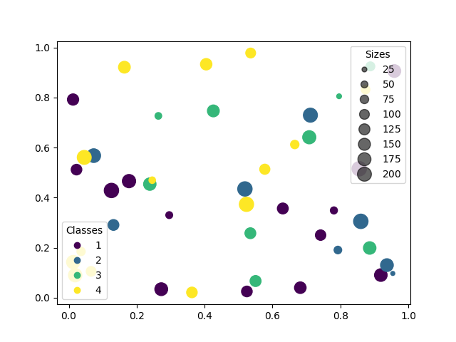
Automated legend creation

Another option for creating a legend for a scatter is to use the PathCollection's legend_elements() method. It will automatically try to determine a useful number of legend entries to be shown and return a tuple of handles and labels. Those can be passed to the call to legend().

N = 45
x, y = np.random.rand(2, N)
c = np.random.randint(1, 5, size=N)
s = np.random.randint(10, 220, size=N)

fig, ax = plt.subplots()

scatter = ax.scatter(x, y, c=c, s=s)

# produce a legend with the unique colors from the scatter
legend1 = ax.legend(*scatter.legend_elements(),
                    loc="lower left", title="Classes")
ax.add_artist(legend1)

# produce a legend with a cross section of sizes from the scatter
handles, labels = scatter.legend_elements(prop="sizes", alpha=0.6)
legend2 = ax.legend(handles, labels, loc="upper right", title="Sizes")

plt.show()

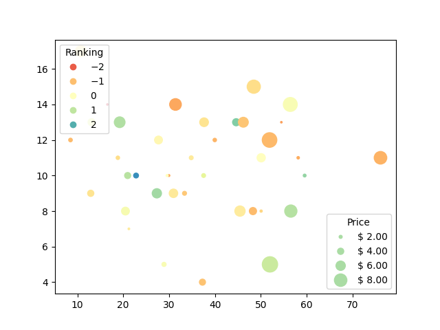
Further arguments to the legend_elements() method can be used to steer how many legend entries are to be created and how they should be labeled. The following shows how to use some of them.

volume = np.random.rayleigh(27, size=40)
amount = np.random.poisson(10, size=40)
ranking = np.random.normal(size=40)
price = np.random.uniform(1, 10, size=40)

fig, ax = plt.subplots()

# Because the price is much too small when being provided as size for ``s``,
# we normalize it to some useful point sizes, s=0.3*(price*3)**2
scatter = ax.scatter(volume, amount, c=ranking, s=0.3*(price*3)**2,
                     vmin=-3, vmax=3, cmap="Spectral")

# Produce a legend for the ranking (colors). Even though there are 40 different
# rankings, we only want to show 5 of them in the legend.
legend1 = ax.legend(*scatter.legend_elements(num=5),
                    loc="upper left", title="Ranking")
ax.add_artist(legend1)

# Produce a legend for the price (sizes). Because we want to show the prices
# in dollars, we use the *func* argument to supply the inverse of the function
# used to calculate the sizes from above. The *fmt* ensures to show the price
# in dollars. Note how we target at 5 elements here, but obtain only 4 in the
# created legend due to the automatic round prices that are chosen for us.
kw = dict(prop="sizes", num=5, color=scatter.cmap(0.7), fmt="$ {x:.2f}",
          func=lambda s: np.sqrt(s/.3)/3)
legend2 = ax.legend(*scatter.legend_elements(**kw),
                    loc="lower right", title="Price")

plt.show()

---

References

The usage of the following functions and methods is shown in this example:

import matplotlib
matplotlib.axes.Axes.scatter
matplotlib.pyplot.scatter
matplotlib.axes.Axes.legend
matplotlib.pyplot.legend
matplotlib.collections.PathCollection.legend_elements

Out:

<function PathCollection.legend_elements at 0x7f154dbc3700>