Version 3.0.3
Note
Click here to download the full example code
Matplotlib has a number of built-in colormaps accessible via
matplotlib.cm.get_cmap. There are also external libraries like
palettable that have many extra colormaps.
However, we often want to create or manipulate colormaps in Matplotlib.
This can be done using the class ListedColormap and a Nx4 numpy array of
values between 0 and 1 to represent the RGBA values of the colormap. There
is also a LinearSegmentedColormap class that allows colormaps to be
specified with a few anchor points defining segments, and linearly
interpolating between the anchor points.
First, getting a named colormap, most of which are listed in
Choosing Colormaps in Matplotlib requires the use of
matplotlib.cm.get_cmap, which returns a
matplotlib.colors.ListedColormap object. The second argument gives
the size of the list of colors used to define the colormap, and below we
use a modest value of 12 so there are not a lot of values to look at.
import numpy as np
import matplotlib as mpl
import matplotlib.pyplot as plt
from matplotlib import cm
from matplotlib.colors import ListedColormap, LinearSegmentedColormap
from collections import OrderedDict

viridis = cm.get_cmap('viridis', 12)
print(viridis)
Out:
<matplotlib.colors.ListedColormap object at 0x7f8697b46668>
The object viridis is a callable, that when passed a float between
0 and 1 returns an RGBA value from the colormap:
print(viridis(0.56))
Out:
(0.119512, 0.607464, 0.540218, 1.0)
The list of colors that comprise the colormap can be directly accessed using
the colors property,
or it can be acccessed indirectly by calling viridis with an array
of values matching the length of the colormap. Note that the returned list
is in the form of an RGBA Nx4 array, where N is the length of the colormap.
print('viridis.colors', viridis.colors)
print('viridis(range(12))', viridis(range(12)))
print('viridis(np.linspace(0, 1, 12))', viridis(np.linspace(0, 1, 12)))
Out:
viridis.colors [[0.267004 0.004874 0.329415 1.      ]
 [0.283072 0.130895 0.449241 1.      ]
 [0.262138 0.242286 0.520837 1.      ]
 [0.220057 0.343307 0.549413 1.      ]
 [0.177423 0.437527 0.557565 1.      ]
 [0.143343 0.522773 0.556295 1.      ]
 [0.119512 0.607464 0.540218 1.      ]
 [0.166383 0.690856 0.496502 1.      ]
 [0.319809 0.770914 0.411152 1.      ]
 [0.525776 0.833491 0.288127 1.      ]
 [0.762373 0.876424 0.137064 1.      ]
 [0.993248 0.906157 0.143936 1.      ]]
viridis(range(12)) [[0.267004 0.004874 0.329415 1.      ]
 [0.283072 0.130895 0.449241 1.      ]
 [0.262138 0.242286 0.520837 1.      ]
 [0.220057 0.343307 0.549413 1.      ]
 [0.177423 0.437527 0.557565 1.      ]
 [0.143343 0.522773 0.556295 1.      ]
 [0.119512 0.607464 0.540218 1.      ]
 [0.166383 0.690856 0.496502 1.      ]
 [0.319809 0.770914 0.411152 1.      ]
 [0.525776 0.833491 0.288127 1.      ]
 [0.762373 0.876424 0.137064 1.      ]
 [0.993248 0.906157 0.143936 1.      ]]
viridis(np.linspace(0, 1, 12)) [[0.267004 0.004874 0.329415 1.      ]
 [0.283072 0.130895 0.449241 1.      ]
 [0.262138 0.242286 0.520837 1.      ]
 [0.220057 0.343307 0.549413 1.      ]
 [0.177423 0.437527 0.557565 1.      ]
 [0.143343 0.522773 0.556295 1.      ]
 [0.119512 0.607464 0.540218 1.      ]
 [0.166383 0.690856 0.496502 1.      ]
 [0.319809 0.770914 0.411152 1.      ]
 [0.525776 0.833491 0.288127 1.      ]
 [0.762373 0.876424 0.137064 1.      ]
 [0.993248 0.906157 0.143936 1.      ]]
The colormap is a lookup table, so "oversampling" the colormap returns nearest-neighbor interpolation (note the repeated colors in the list below)
print('viridis(np.linspace(0, 1, 15))', viridis(np.linspace(0, 1, 15)))
Out:
viridis(np.linspace(0, 1, 15)) [[0.267004 0.004874 0.329415 1.      ]
 [0.267004 0.004874 0.329415 1.      ]
 [0.283072 0.130895 0.449241 1.      ]
 [0.262138 0.242286 0.520837 1.      ]
 [0.220057 0.343307 0.549413 1.      ]
 [0.177423 0.437527 0.557565 1.      ]
 [0.143343 0.522773 0.556295 1.      ]
 [0.119512 0.607464 0.540218 1.      ]
 [0.119512 0.607464 0.540218 1.      ]
 [0.166383 0.690856 0.496502 1.      ]
 [0.319809 0.770914 0.411152 1.      ]
 [0.525776 0.833491 0.288127 1.      ]
 [0.762373 0.876424 0.137064 1.      ]
 [0.993248 0.906157 0.143936 1.      ]
 [0.993248 0.906157 0.143936 1.      ]]
This is essential the inverse operation of the above where we supply a
Nx4 numpy array with all values between 0 and 1,
to ListedColormap to make a new colormap. This means that
any numpy operations that we can do on a Nx4 array make carpentry of
new colormaps from existing colormaps quite straight forward.
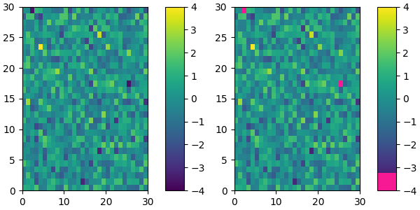
Suppose we want to make the first 25 entries of a 256-length "viridis" colormap pink for some reason:
viridis = cm.get_cmap('viridis', 256)
newcolors = viridis(np.linspace(0, 1, 256))
pink = np.array([248/256, 24/256, 148/256, 1])
newcolors[:25, :] = pink
newcmp = ListedColormap(newcolors)


def plot_examples(cms):
    """
    helper function to plot two colormaps
    """
    np.random.seed(19680801)
    data = np.random.randn(30, 30)

    fig, axs = plt.subplots(1, 2, figsize=(6, 3), constrained_layout=True)
    for [ax, cmap] in zip(axs, cms):
        psm = ax.pcolormesh(data, cmap=cmap, rasterized=True, vmin=-4, vmax=4)
        fig.colorbar(psm, ax=ax)
    plt.show()

plot_examples([viridis, newcmp])
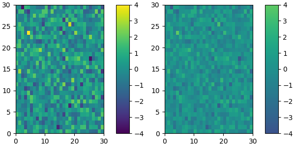
We can easily reduce the dynamic range of a colormap; here we choose the middle 0.5 of the colormap. However, we need to interpolate from a larger colormap, otherwise the new colormap will have repeated values.
viridisBig = cm.get_cmap('viridis', 512)
newcmp = ListedColormap(viridisBig(np.linspace(0.25, 0.75, 256)))
plot_examples([viridis, newcmp])
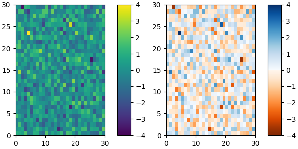
and we can easily concatenate two colormaps:
top = cm.get_cmap('Oranges_r', 128)
bottom = cm.get_cmap('Blues', 128)

newcolors = np.vstack((top(np.linspace(0, 1, 128)),
                       bottom(np.linspace(0, 1, 128))))
newcmp = ListedColormap(newcolors, name='OrangeBlue')
plot_examples([viridis, newcmp])
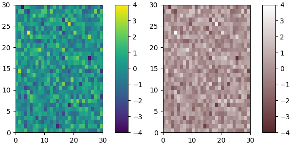
Of course we need not start from a named colormap, we just need to create
the Nx4 array to pass to ListedColormap. Here we create a
brown colormap that goes to white....
N = 256
vals = np.ones((N, 4))
vals[:, 0] = np.linspace(90/256, 1, N)
vals[:, 1] = np.linspace(39/256, 1, N)
vals[:, 2] = np.linspace(41/256, 1, N)
newcmp = ListedColormap(vals)
plot_examples([viridis, newcmp])
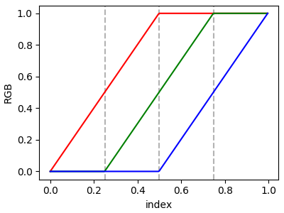
LinearSegmentedColormap class specifies colormaps using anchor points
between which RGB(A) values are interpolated.
The format to specify these colormaps allows discontinuities at the anchor
points. Each anchor point is specified as a row in a matrix of the
form [x[i] yleft[i] yright[i]], where x[i] is the anchor, and
yleft[i] and yright[i] are the values of the color on either
side of the anchor point.
If there are no discontinuities, then yleft[i]=yright[i]:
cdict = {'red':   [[0.0,  0.0, 0.0],
                   [0.5,  1.0, 1.0],
                   [1.0,  1.0, 1.0]],
         'green': [[0.0,  0.0, 0.0],
                   [0.25, 0.0, 0.0],
                   [0.75, 1.0, 1.0],
                   [1.0,  1.0, 1.0]],
         'blue':  [[0.0,  0.0, 0.0],
                   [0.5,  0.0, 0.0],
                   [1.0,  1.0, 1.0]]}


def plot_linearmap(cdict):
    newcmp = LinearSegmentedColormap('testCmap', segmentdata=cdict, N=256)
    rgba = newcmp(np.linspace(0, 1, 256))
    fig, ax = plt.subplots(figsize=(4, 3), constrained_layout=True)
    col = ['r', 'g', 'b']
    for xx in [0.25, 0.5, 0.75]:
        ax.axvline(xx, color='0.7', linestyle='--')
    for i in range(3):
        ax.plot(np.arange(256)/256, rgba[:, i], color=col[i])
    ax.set_xlabel('index')
    ax.set_ylabel('RGB')
    plt.show()

plot_linearmap(cdict)
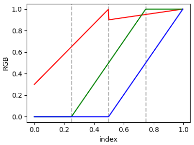
In order to make a discontinuity at an anchor point, the third column is different than the second. The matrix for each of "red", "green", "blue", and optionally "alpha" is set up as:
cdict['red'] = [...
                [x[i]      yleft[i]     yright[i]],
                [x[i+1]    yleft[i+1]   yright[i+1]],
               ...]
and for values passed to the colormap between x[i] and x[i+1],
the interpolation is between yright[i] and yleft[i+1].
In the example below there is a discontiuity in red at 0.5. The interpolation between 0 and 0.5 goes from 0.3 to 1, and between 0.5 and 1 it goes from 0.9 to 1. Note that red[0, 1], and red[2, 2] are both superfluous to the interpolation because red[0, 1] is the value to the left of 0, and red[2, 2] is the value to the right of 1.0.
cdict['red'] = [[0.0,  0.0, 0.3],
                [0.5,  1.0, 0.9],
                [1.0,  1.0, 1.0]]
plot_linearmap(cdict)
The use of the following functions, methods, classes and modules is shown in this example:
Keywords: matplotlib code example, codex, python plot, pyplot Gallery generated by Sphinx-Gallery