Version 3.0.3
Note
Click here to download the full example code
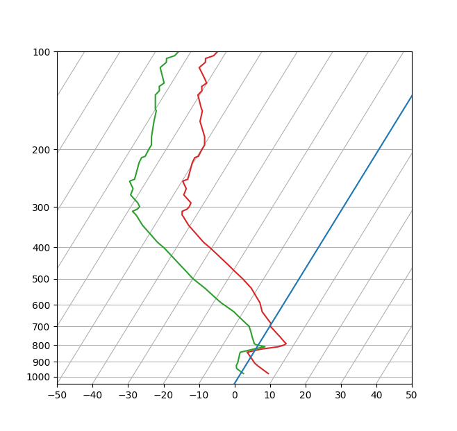
This serves as an intensive exercise of matplotlib's transforms and custom projection API. This example produces a so-called SkewT-logP diagram, which is a common plot in meteorology for displaying vertical profiles of temperature. As far as matplotlib is concerned, the complexity comes from having X and Y axes that are not orthogonal. This is handled by including a skew component to the basic Axes transforms. Additional complexity comes in handling the fact that the upper and lower X-axes have different data ranges, which necessitates a bunch of custom classes for ticks,spines, and the axis to handle this.
from matplotlib.axes import Axes
import matplotlib.transforms as transforms
import matplotlib.axis as maxis
import matplotlib.spines as mspines
from matplotlib.projections import register_projection


# The sole purpose of this class is to look at the upper, lower, or total
# interval as appropriate and see what parts of the tick to draw, if any.
class SkewXTick(maxis.XTick):
    def update_position(self, loc):
        # This ensures that the new value of the location is set before
        # any other updates take place
        self._loc = loc
        super().update_position(loc)

    def _has_default_loc(self):
        return self.get_loc() is None

    def _need_lower(self):
        return (self._has_default_loc() or
                transforms.interval_contains(self.axes.lower_xlim,
                                             self.get_loc()))

    def _need_upper(self):
        return (self._has_default_loc() or
                transforms.interval_contains(self.axes.upper_xlim,
                                             self.get_loc()))

    @property
    def gridOn(self):
        return (self._gridOn and (self._has_default_loc() or
                transforms.interval_contains(self.get_view_interval(),
                                             self.get_loc())))

    @gridOn.setter
    def gridOn(self, value):
        self._gridOn = value

    @property
    def tick1On(self):
        return self._tick1On and self._need_lower()

    @tick1On.setter
    def tick1On(self, value):
        self._tick1On = value

    @property
    def label1On(self):
        return self._label1On and self._need_lower()

    @label1On.setter
    def label1On(self, value):
        self._label1On = value

    @property
    def tick2On(self):
        return self._tick2On and self._need_upper()

    @tick2On.setter
    def tick2On(self, value):
        self._tick2On = value

    @property
    def label2On(self):
        return self._label2On and self._need_upper()

    @label2On.setter
    def label2On(self, value):
        self._label2On = value

    def get_view_interval(self):
        return self.axes.xaxis.get_view_interval()


# This class exists to provide two separate sets of intervals to the tick,
# as well as create instances of the custom tick
class SkewXAxis(maxis.XAxis):
    def _get_tick(self, major):
        return SkewXTick(self.axes, None, '', major=major)

    def get_view_interval(self):
        return self.axes.upper_xlim[0], self.axes.lower_xlim[1]


# This class exists to calculate the separate data range of the
# upper X-axis and draw the spine there. It also provides this range
# to the X-axis artist for ticking and gridlines
class SkewSpine(mspines.Spine):
    def _adjust_location(self):
        pts = self._path.vertices
        if self.spine_type == 'top':
            pts[:, 0] = self.axes.upper_xlim
        else:
            pts[:, 0] = self.axes.lower_xlim


# This class handles registration of the skew-xaxes as a projection as well
# as setting up the appropriate transformations. It also overrides standard
# spines and axes instances as appropriate.
class SkewXAxes(Axes):
    # The projection must specify a name.  This will be used be the
    # user to select the projection, i.e. ``subplot(111,
    # projection='skewx')``.
    name = 'skewx'

    def _init_axis(self):
        # Taken from Axes and modified to use our modified X-axis
        self.xaxis = SkewXAxis(self)
        self.spines['top'].register_axis(self.xaxis)
        self.spines['bottom'].register_axis(self.xaxis)
        self.yaxis = maxis.YAxis(self)
        self.spines['left'].register_axis(self.yaxis)
        self.spines['right'].register_axis(self.yaxis)

    def _gen_axes_spines(self):
        spines = {'top': SkewSpine.linear_spine(self, 'top'),
                  'bottom': mspines.Spine.linear_spine(self, 'bottom'),
                  'left': mspines.Spine.linear_spine(self, 'left'),
                  'right': mspines.Spine.linear_spine(self, 'right')}
        return spines

    def _set_lim_and_transforms(self):
        """
        This is called once when the plot is created to set up all the
        transforms for the data, text and grids.
        """
        rot = 30

        # Get the standard transform setup from the Axes base class
        Axes._set_lim_and_transforms(self)

        # Need to put the skew in the middle, after the scale and limits,
        # but before the transAxes. This way, the skew is done in Axes
        # coordinates thus performing the transform around the proper origin
        # We keep the pre-transAxes transform around for other users, like the
        # spines for finding bounds
        self.transDataToAxes = self.transScale + \
            self.transLimits + transforms.Affine2D().skew_deg(rot, 0)

        # Create the full transform from Data to Pixels
        self.transData = self.transDataToAxes + self.transAxes

        # Blended transforms like this need to have the skewing applied using
        # both axes, in axes coords like before.
        self._xaxis_transform = (transforms.blended_transform_factory(
            self.transScale + self.transLimits,
            transforms.IdentityTransform()) +
            transforms.Affine2D().skew_deg(rot, 0)) + self.transAxes

    @property
    def lower_xlim(self):
        return self.axes.viewLim.intervalx

    @property
    def upper_xlim(self):
        pts = [[0., 1.], [1., 1.]]
        return self.transDataToAxes.inverted().transform(pts)[:, 0]


# Now register the projection with matplotlib so the user can select
# it.
register_projection(SkewXAxes)

if __name__ == '__main__':
    # Now make a simple example using the custom projection.
    from io import StringIO
    from matplotlib.ticker import (MultipleLocator, NullFormatter,
                                   ScalarFormatter)
    import matplotlib.pyplot as plt
    import numpy as np

    # Some examples data
    data_txt = '''
  978.0    345    7.8    0.8     61   4.16    325     14  282.7  294.6  283.4
  971.0    404    7.2    0.2     61   4.01    327     17  282.7  294.2  283.4
  946.7    610    5.2   -1.8     61   3.56    335     26  282.8  293.0  283.4
  944.0    634    5.0   -2.0     61   3.51    336     27  282.8  292.9  283.4
  925.0    798    3.4   -2.6     65   3.43    340     32  282.8  292.7  283.4
  911.8    914    2.4   -2.7     69   3.46    345     37  282.9  292.9  283.5
  906.0    966    2.0   -2.7     71   3.47    348     39  283.0  293.0  283.6
  877.9   1219    0.4   -3.2     77   3.46      0     48  283.9  293.9  284.5
  850.0   1478   -1.3   -3.7     84   3.44      0     47  284.8  294.8  285.4
  841.0   1563   -1.9   -3.8     87   3.45    358     45  285.0  295.0  285.6
  823.0   1736    1.4   -0.7     86   4.44    353     42  290.3  303.3  291.0
  813.6   1829    4.5    1.2     80   5.17    350     40  294.5  309.8  295.4
  809.0   1875    6.0    2.2     77   5.57    347     39  296.6  313.2  297.6
  798.0   1988    7.4   -0.6     57   4.61    340     35  299.2  313.3  300.1
  791.0   2061    7.6   -1.4     53   4.39    335     33  300.2  313.6  301.0
  783.9   2134    7.0   -1.7     54   4.32    330     31  300.4  313.6  301.2
  755.1   2438    4.8   -3.1     57   4.06    300     24  301.2  313.7  301.9
  727.3   2743    2.5   -4.4     60   3.81    285     29  301.9  313.8  302.6
  700.5   3048    0.2   -5.8     64   3.57    275     31  302.7  313.8  303.3
  700.0   3054    0.2   -5.8     64   3.56    280     31  302.7  313.8  303.3
  698.0   3077    0.0   -6.0     64   3.52    280     31  302.7  313.7  303.4
  687.0   3204   -0.1   -7.1     59   3.28    281     31  304.0  314.3  304.6
  648.9   3658   -3.2  -10.9     55   2.59    285     30  305.5  313.8  305.9
  631.0   3881   -4.7  -12.7     54   2.29    289     33  306.2  313.6  306.6
  600.7   4267   -6.4  -16.7     44   1.73    295     39  308.6  314.3  308.9
  592.0   4381   -6.9  -17.9     41   1.59    297     41  309.3  314.6  309.6
  577.6   4572   -8.1  -19.6     39   1.41    300     44  310.1  314.9  310.3
  555.3   4877  -10.0  -22.3     36   1.16    295     39  311.3  315.3  311.5
  536.0   5151  -11.7  -24.7     33   0.97    304     39  312.4  315.8  312.6
  533.8   5182  -11.9  -25.0     33   0.95    305     39  312.5  315.8  312.7
  500.0   5680  -15.9  -29.9     29   0.64    290     44  313.6  315.9  313.7
  472.3   6096  -19.7  -33.4     28   0.49    285     46  314.1  315.8  314.1
  453.0   6401  -22.4  -36.0     28   0.39    300     50  314.4  315.8  314.4
  400.0   7310  -30.7  -43.7     27   0.20    285     44  315.0  315.8  315.0
  399.7   7315  -30.8  -43.8     27   0.20    285     44  315.0  315.8  315.0
  387.0   7543  -33.1  -46.1     26   0.16    281     47  314.9  315.5  314.9
  382.7   7620  -33.8  -46.8     26   0.15    280     48  315.0  315.6  315.0
  342.0   8398  -40.5  -53.5     23   0.08    293     52  316.1  316.4  316.1
  320.4   8839  -43.7  -56.7     22   0.06    300     54  317.6  317.8  317.6
  318.0   8890  -44.1  -57.1     22   0.05    301     55  317.8  318.0  317.8
  310.0   9060  -44.7  -58.7     19   0.04    304     61  319.2  319.4  319.2
  306.1   9144  -43.9  -57.9     20   0.05    305     63  321.5  321.7  321.5
  305.0   9169  -43.7  -57.7     20   0.05    303     63  322.1  322.4  322.1
  300.0   9280  -43.5  -57.5     20   0.05    295     64  323.9  324.2  323.9
  292.0   9462  -43.7  -58.7     17   0.05    293     67  326.2  326.4  326.2
  276.0   9838  -47.1  -62.1     16   0.03    290     74  326.6  326.7  326.6
  264.0  10132  -47.5  -62.5     16   0.03    288     79  330.1  330.3  330.1
  251.0  10464  -49.7  -64.7     16   0.03    285     85  331.7  331.8  331.7
  250.0  10490  -49.7  -64.7     16   0.03    285     85  332.1  332.2  332.1
  247.0  10569  -48.7  -63.7     16   0.03    283     88  334.7  334.8  334.7
  244.0  10649  -48.9  -63.9     16   0.03    280     91  335.6  335.7  335.6
  243.3  10668  -48.9  -63.9     16   0.03    280     91  335.8  335.9  335.8
  220.0  11327  -50.3  -65.3     15   0.03    280     85  343.5  343.6  343.5
  212.0  11569  -50.5  -65.5     15   0.03    280     83  346.8  346.9  346.8
  210.0  11631  -49.7  -64.7     16   0.03    280     83  349.0  349.1  349.0
  200.0  11950  -49.9  -64.9     15   0.03    280     80  353.6  353.7  353.6
  194.0  12149  -49.9  -64.9     15   0.03    279     78  356.7  356.8  356.7
  183.0  12529  -51.3  -66.3     15   0.03    278     75  360.4  360.5  360.4
  164.0  13233  -55.3  -68.3     18   0.02    277     69  365.2  365.3  365.2
  152.0  13716  -56.5  -69.5     18   0.02    275     65  371.1  371.2  371.1
  150.0  13800  -57.1  -70.1     18   0.02    275     64  371.5  371.6  371.5
  136.0  14414  -60.5  -72.5     19   0.02    268     54  376.0  376.1  376.0
  132.0  14600  -60.1  -72.1     19   0.02    265     51  380.0  380.1  380.0
  131.4  14630  -60.2  -72.2     19   0.02    265     51  380.3  380.4  380.3
  128.0  14792  -60.9  -72.9     19   0.02    266     50  381.9  382.0  381.9
  125.0  14939  -60.1  -72.1     19   0.02    268     49  385.9  386.0  385.9
  119.0  15240  -62.2  -73.8     20   0.01    270     48  387.4  387.5  387.4
  112.0  15616  -64.9  -75.9     21   0.01    265     53  389.3  389.3  389.3
  108.0  15838  -64.1  -75.1     21   0.01    265     58  394.8  394.9  394.8
  107.8  15850  -64.1  -75.1     21   0.01    265     58  395.0  395.1  395.0
  105.0  16010  -64.7  -75.7     21   0.01    272     50  396.9  396.9  396.9
  103.0  16128  -62.9  -73.9     21   0.02    277     45  402.5  402.6  402.5
  100.0  16310  -62.5  -73.5     21   0.02    285     36  406.7  406.8  406.7
    '''

    # Parse the data
    sound_data = StringIO(data_txt)
    p, h, T, Td = np.loadtxt(sound_data, usecols=range(0, 4), unpack=True)

    # Create a new figure. The dimensions here give a good aspect ratio
    fig = plt.figure(figsize=(6.5875, 6.2125))
    ax = fig.add_subplot(111, projection='skewx')

    plt.grid(True)

    # Plot the data using normal plotting functions, in this case using
    # log scaling in Y, as dictated by the typical meteorological plot
    ax.semilogy(T, p, color='C3')
    ax.semilogy(Td, p, color='C2')

    # An example of a slanted line at constant X
    l = ax.axvline(0, color='C0')

    # Disables the log-formatting that comes with semilogy
    ax.yaxis.set_major_formatter(ScalarFormatter())
    ax.yaxis.set_minor_formatter(NullFormatter())
    ax.set_yticks(np.linspace(100, 1000, 10))
    ax.set_ylim(1050, 100)

    ax.xaxis.set_major_locator(MultipleLocator(10))
    ax.set_xlim(-50, 50)

    plt.show()
The use of the following functions, methods, classes and modules is shown in this example:
Keywords: matplotlib code example, codex, python plot, pyplot Gallery generated by Sphinx-Gallery