Version 2.2.0
Objects that use colormaps by default linearly map the colors in the colormap from data values vmin to vmax. For example:
pcm = ax.pcolormesh(x, y, Z, vmin=-1., vmax=1., cmap='RdBu_r')
will map the data in Z linearly from -1 to +1, so Z=0 will give a color at the center of the colormap RdBu_r (white in this case).
Matplotlib does this mapping in two steps, with a normalization from
[0,1] occurring first, and then mapping onto the indices in the
colormap. Normalizations are classes defined in the
matplotlib.colors() module. The default, linear normalization is
matplotlib.colors.Normalize().
Artists that map data to color pass the arguments vmin and vmax to
construct a matplotlib.colors.Normalize() instance, then call it:
In [1]: import matplotlib as mpl

In [2]: norm = mpl.colors.Normalize(vmin=-1.,vmax=1.)

In [3]: norm(0.)
Out[3]: 0.5
However, there are sometimes cases where it is useful to map data to colormaps in a non-linear fashion.
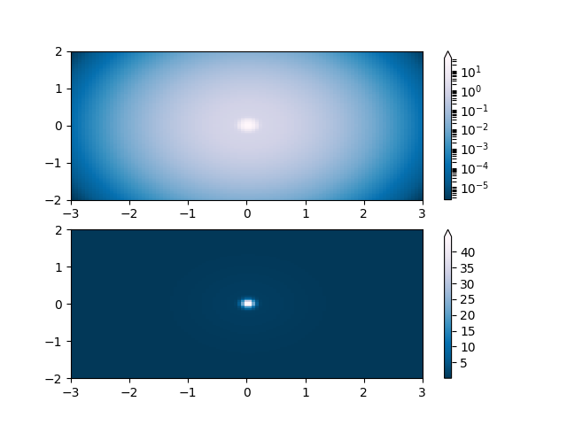
One of the most common transformations is to plot data by taking
its logarithm (to the base-10). This transformation is useful to
display changes across disparate scales. Using colors.LogNorm()
normalizes the data via  . In the example below,
there are two bumps, one much smaller than the other. Using
. In the example below,
there are two bumps, one much smaller than the other. Using
colors.LogNorm(), the shape and location of each bump can clearly
be seen:
import numpy as np
import matplotlib.pyplot as plt
import matplotlib.colors as colors

N = 100
X, Y = np.mgrid[-3:3:complex(0, N), -2:2:complex(0, N)]

# A low hump with a spike coming out of the top right.  Needs to have
# z/colour axis on a log scale so we see both hump and spike.  linear
# scale only shows the spike.
Z1 = np.exp(-(X)**2 - (Y)**2)
Z2 = np.exp(-(X * 10)**2 - (Y * 10)**2)
Z = Z1 + 50 * Z2

fig, ax = plt.subplots(2, 1)

pcm = ax[0].pcolor(X, Y, Z,
                   norm=colors.LogNorm(vmin=Z.min(), vmax=Z.max()),
                   cmap='PuBu_r')
fig.colorbar(pcm, ax=ax[0], extend='max')

pcm = ax[1].pcolor(X, Y, Z, cmap='PuBu_r')
fig.colorbar(pcm, ax=ax[1], extend='max')
fig.show()
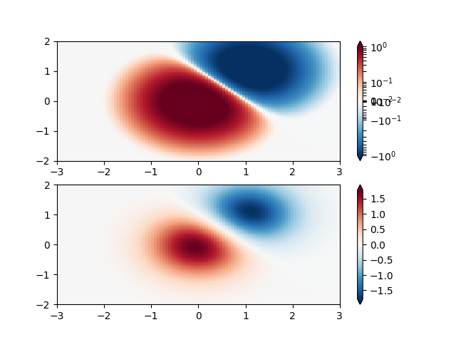
Similarly, it sometimes happens that there is data that is positive
and negative, but we would still like a logarithmic scaling applied to
both. In this case, the negative numbers are also scaled
logarithmically, and mapped to smaller numbers; e.g., if vmin=-vmax,
then they the negative numbers are mapped from 0 to 0.5 and the
positive from 0.5 to 1.
Since the logarithm of values close to zero tends toward infinity, a small range around zero needs to be mapped linearly. The parameter linthresh allows the user to specify the size of this range (-linthresh, linthresh). The size of this range in the colormap is set by linscale. When linscale == 1.0 (the default), the space used for the positive and negative halves of the linear range will be equal to one decade in the logarithmic range.
N = 100
X, Y = np.mgrid[-3:3:complex(0, N), -2:2:complex(0, N)]
Z1 = np.exp(-X**2 - Y**2)
Z2 = np.exp(-(X - 1)**2 - (Y - 1)**2)
Z = (Z1 - Z2) * 2

fig, ax = plt.subplots(2, 1)

pcm = ax[0].pcolormesh(X, Y, Z,
                       norm=colors.SymLogNorm(linthresh=0.03, linscale=0.03,
                                              vmin=-1.0, vmax=1.0),
                       cmap='RdBu_r')
fig.colorbar(pcm, ax=ax[0], extend='both')

pcm = ax[1].pcolormesh(X, Y, Z, cmap='RdBu_r', vmin=-np.max(Z))
fig.colorbar(pcm, ax=ax[1], extend='both')
fig.show()
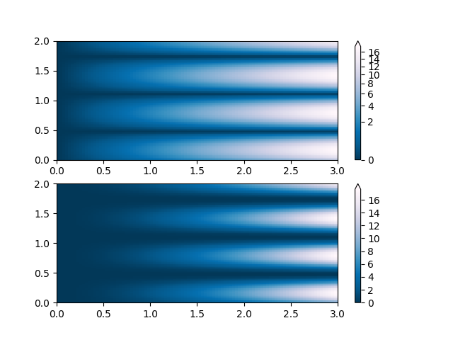
Sometimes it is useful to remap the colors onto a power-law
relationship (i.e.  , where
  is the
power). For this we use the
is the
power). For this we use the colors.PowerNorm(). It takes as an
argument gamma (gamma == 1.0 will just yield the default linear
normalization):
Note
There should probably be a good reason for plotting the data using this type of transformation. Technical viewers are used to linear and logarithmic axes and data transformations. Power laws are less common, and viewers should explicitly be made aware that they have been used.
N = 100
X, Y = np.mgrid[0:3:complex(0, N), 0:2:complex(0, N)]
Z1 = (1 + np.sin(Y * 10.)) * X**(2.)

fig, ax = plt.subplots(2, 1)

pcm = ax[0].pcolormesh(X, Y, Z1, norm=colors.PowerNorm(gamma=0.5),
                       cmap='PuBu_r')
fig.colorbar(pcm, ax=ax[0], extend='max')

pcm = ax[1].pcolormesh(X, Y, Z1, cmap='PuBu_r')
fig.colorbar(pcm, ax=ax[1], extend='max')
fig.show()
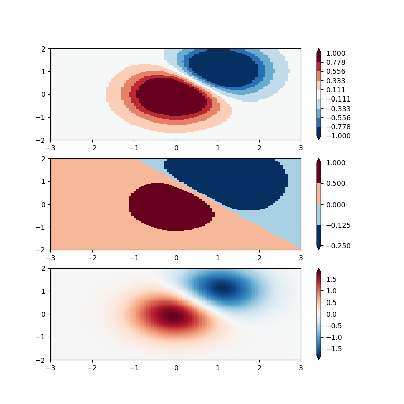
Another normaization that comes with matplolib is
colors.BoundaryNorm(). In addition to vmin and vmax, this
takes as arguments boundaries between which data is to be mapped. The
colors are then linearly distributed between these “bounds”. For
instance:
In [4]: import matplotlib.colors as colors

In [5]: bounds = np.array([-0.25, -0.125, 0, 0.5, 1])

In [6]: norm = colors.BoundaryNorm(boundaries=bounds, ncolors=4)

In [7]: print(norm([-0.2,-0.15,-0.02, 0.3, 0.8, 0.99]))
[0 0 1 2 3 3]
Note unlike the other norms, this norm returns values from 0 to ncolors-1.
N = 100
X, Y = np.mgrid[-3:3:complex(0, N), -2:2:complex(0, N)]
Z1 = np.exp(-X**2 - Y**2)
Z2 = np.exp(-(X - 1)**2 - (Y - 1)**2)
Z = (Z1 - Z2) * 2

fig, ax = plt.subplots(3, 1, figsize=(8, 8))
ax = ax.flatten()
# even bounds gives a contour-like effect
bounds = np.linspace(-1, 1, 10)
norm = colors.BoundaryNorm(boundaries=bounds, ncolors=256)
pcm = ax[0].pcolormesh(X, Y, Z,
                       norm=norm,
                       cmap='RdBu_r')
fig.colorbar(pcm, ax=ax[0], extend='both', orientation='vertical')

# uneven bounds changes the colormapping:
bounds = np.array([-0.25, -0.125, 0, 0.5, 1])
norm = colors.BoundaryNorm(boundaries=bounds, ncolors=256)
pcm = ax[1].pcolormesh(X, Y, Z, norm=norm, cmap='RdBu_r')
fig.colorbar(pcm, ax=ax[1], extend='both', orientation='vertical')

pcm = ax[2].pcolormesh(X, Y, Z, cmap='RdBu_r', vmin=-np.max(Z))
fig.colorbar(pcm, ax=ax[2], extend='both', orientation='vertical')
fig.show()
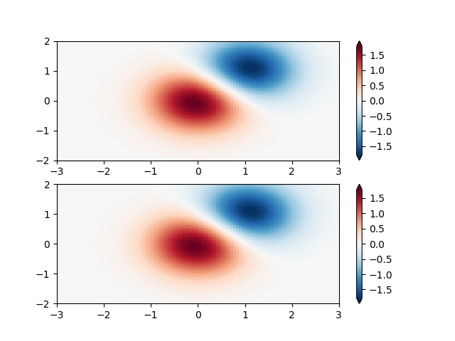
It is possible to define your own normalization. In the following
example, we modify colors:SymLogNorm() to use different linear
maps for the negative data values and the positive. (Note that this
example is simple, and does not validate inputs or account for complex
cases such as masked data)
Note
This may appear soon as colors.OffsetNorm().
As above, non-symmetric mapping of data to color is non-standard practice for quantitative data, and should only be used advisedly. A practical example is having an ocean/land colormap where the land and ocean data span different ranges.
N = 100
X, Y = np.mgrid[-3:3:complex(0, N), -2:2:complex(0, N)]
Z1 = np.exp(-X**2 - Y**2)
Z2 = np.exp(-(X - 1)**2 - (Y - 1)**2)
Z = (Z1 - Z2) * 2


class MidpointNormalize(colors.Normalize):
    def __init__(self, vmin=None, vmax=None, midpoint=None, clip=False):
        self.midpoint = midpoint
        colors.Normalize.__init__(self, vmin, vmax, clip)

    def __call__(self, value, clip=None):
        # I'm ignoring masked values and all kinds of edge cases to make a
        # simple example...
        x, y = [self.vmin, self.midpoint, self.vmax], [0, 0.5, 1]
        return np.ma.masked_array(np.interp(value, x, y))


fig, ax = plt.subplots(2, 1)

pcm = ax[0].pcolormesh(X, Y, Z,
                       norm=MidpointNormalize(midpoint=0.),
                       cmap='RdBu_r')
fig.colorbar(pcm, ax=ax[0], extend='both')

pcm = ax[1].pcolormesh(X, Y, Z, cmap='RdBu_r', vmin=-np.max(Z))
fig.colorbar(pcm, ax=ax[1], extend='both')
fig.show()