
The most important changes in matplotlib 2.0 are the changes to the default style.
While it is impossible to select the best default for all cases, these are designed to work well in the most common cases.
A ‘classic’ style sheet is provided so reverting to the 1.x default values is a single line of python
import matplotlib.style
import matplotlib as mpl
mpl.style.use('classic')
See The matplotlibrc file for details about how to persistently and selectively revert many of these changes.
Table of Contents
The colors in the default property cycle have been changed from
['b', 'g', 'r', 'c', 'm', 'y', 'k'] to the category10
color palette used by Vega and
d3
originally developed at Tableau.
(Source code, png, pdf)
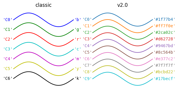
In addition to changing the colors, an additional method to specify
colors was added. Previously, the default colors were the single
character short-hand notations for red, green, blue, cyan, magenta,
yellow, and black. This made them easy to type and usable in the
abbreviated style string in plot, however the new default colors
are only specified via hex values. To access these colors outside of
the property cycling the notation for colors 'CN', where N
takes values 0-9, was added to
denote the first 10 colors in mpl.rcParams['axes.prop_cycle'] See
Specifying Colors for more details.
To restore the old color cycle use
from cycler import cycler
mpl.rcParams['axes.prop_cycle'] = cycler(color='bgrcmyk')
or set
axes.prop_cycle : cycler('color', 'bgrcmyk')
in your matplotlibrc file.
matplotlib.cm.ScalarMappable instances is'viridis' (aka option D).(Source code, png, pdf)
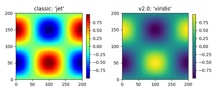
For an introduction to color theory and how ‘viridis’ was generated watch Nathaniel Smith and Stéfan van der Walt’s talk from SciPy2015. See here for many more details about the other alternatives and the tools used to create the color map. For details on all of the color maps available in matplotlib see Colormaps in Matplotlib.
The previous default can be restored using
mpl.rcParams['image.cmap'] = 'jet'
or setting
image.cmap : 'jet'
in your matplotlibrc file; however this is strongly discouraged.
The default interactive figure background color has changed from grey to white, which matches the default background color used when saving.
The previous defaults can be restored by
mpl.rcParams['figure.facecolor'] = '0.75'
or by setting
figure.facecolor : '0.75'
in your matplotlibrc file.
The default style of grid lines was changed from black dashed lines to thicker solid light grey lines.
(Source code, png, pdf)
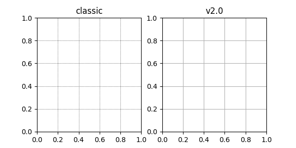
The previous default can be restored by using:
mpl.rcParams['grid.color'] = 'k'
mpl.rcParams['grid.linestyle'] = ':'
mpl.rcParams['grid.linewidth'] = 0.5
or by setting:
grid.color       :   k       # grid color
grid.linestyle   :   :       # dotted
grid.linewidth   :   0.5     # in points
in your matplotlibrc file.
The default dpi used for on-screen display was changed from 80 dpi to
100 dpi, the same as the default dpi for saving files. Due to this
change, the on-screen display is now more what-you-see-is-what-you-get
for saved files. To keep the figure the same size in terms of pixels, in
order to maintain approximately the same size on the screen, the
default figure size was reduced from 8x6 inches to 6.4x4.8 inches. As
a consequence of this the default font sizes used for the title, tick
labels, and axes labels were reduced to maintain their size relative
to the overall size of the figure. By default the dpi of the saved
image is now the dpi of the Figure instance being
saved.
This will have consequences if you are trying to match text in a figure directly with external text.
The previous defaults can be restored by
mpl.rcParams['figure.figsize'] = [8.0, 6.0]
mpl.rcParams['figure.dpi'] = 80
mpl.rcParams['savefig.dpi'] = 100

mpl.rcParams['font.size'] = 12
mpl.rcParams['legend.fontsize'] = 'large'
mpl.rcParams['figure.titlesize'] = 'medium'
or by setting:
figure.figsize   : [8.0, 6.0]
figure.dpi       : 80
savefig.dpi      : 100

font.size        : 12.0
legend.fontsize  : 'large'
figure.titlesize : 'medium'
In your matplotlibrc file.
In addition, the forward kwarg to
set_size_inches now defaults to True to improve
the interactive experience. Backend canvases that adjust the size of
their bound matplotlib.figure.Figure must pass forward=False to
avoid circular behavior. This default is not configurable.
scatter¶The following changes were made to the default behavior of
scatter
- The default size of the elements in a scatter plot is now based on the rcParam
lines.markersizeso it is consistent withplot(X, Y, 'o'). The old value was 20, and the new value is 36 (6^2).- scatter markers no longer have a black edge.
- if the color of the markers is not specified it will follow the property cycle, pulling from the ‘patches’ cycle on the
Axes.
(Source code, png, pdf)
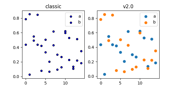
The classic default behavior of scatter can
only be recovered through mpl.style.use('classic'). The marker size
can be recovered via
mpl.rcParam['lines.markersize'] = np.sqrt(20)
however, this will also affect the default marker size of
plot. To recover the classic behavior on
a per-call basis pass the following kwargs:
classic_kwargs = {'s': 20, 'edgecolors': 'k', 'c': 'b'}
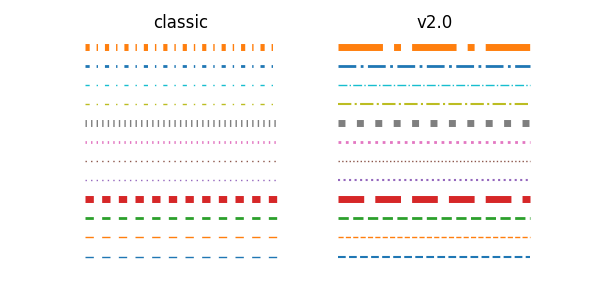
plot¶The following changes were made to the default behavior of
plot
- the default linewidth increased from 1 to 1.5
- the dash patterns associated with
'--',':', and'-.'have changed- the dash patterns now scale with line width
(Source code, png, pdf)

The previous defaults can be restored by setting:
mpl.rcParams['lines.linewidth'] = 1.0
mpl.rcParams['lines.dashed_pattern'] = [6, 6]
mpl.rcParams['lines.dashdot_pattern'] = [3, 5, 1, 5]
mpl.rcParams['lines.dotted_pattern'] = [1, 3]
mpl.rcParams['lines.scale_dashes'] = False
or by setting:
lines.linewidth   : 1.0
lines.dashed_pattern : 6, 6
lines.dashdot_pattern : 3, 5, 1, 5
lines.dotted_pattern : 1, 3
lines.scale_dashes: False
in your matplotlibrc file.
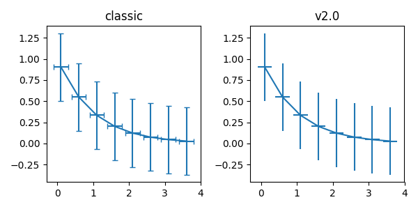
errorbar¶By default, caps on the ends of errorbars are not present.
(Source code, png, pdf)

This also changes the return value of
errorbar() as the list of ‘caplines’ will
be empty by default.
The previous defaults can be restored by setting:
mpl.rcParams['errorbar.capsize'] = 3
or by setting
errorbar.capsize : 3
in your matplotlibrc file.
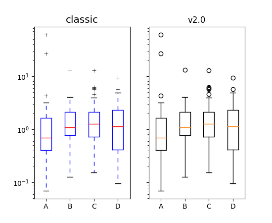
boxplot¶Previously, boxplots were composed of a mish-mash of styles that were, for
better for worse, inherited from Matlab. Most of the elements were blue,
but the medians were red. The fliers (outliers) were black plus-symbols
(+) and the whiskers were dashed lines, which created ambiguity if
the (solid and black) caps were not drawn.
For the new defaults, everything is black except for the median and mean lines (if drawn), which are set to the first two elements of the current color cycle. Also, the default flier markers are now hollow circles, which maintain the ability of the plus-symbols to overlap without obscuring data too much.
(Source code, png, pdf)
The previous defaults can be restored by setting:
mpl.rcParams['boxplot.flierprops.color'] = 'k'
mpl.rcParams['boxplot.flierprops.marker'] = '+'
mpl.rcParams['boxplot.flierprops.markerfacecolor'] = 'none'
mpl.rcParams['boxplot.flierprops.markeredgecolor'] = 'k'
mpl.rcParams['boxplot.boxprops.color'] = 'b'
mpl.rcParams['boxplot.whiskerprops.color'] = 'b'
mpl.rcParams['boxplot.whiskerprops.linestyle'] = '--'
mpl.rcParams['boxplot.medianprops.color'] = 'r'
mpl.rcParams['boxplot.meanprops.color'] = 'r'
mpl.rcParams['boxplot.meanprops.marker'] = '^'
mpl.rcParams['boxplot.meanprops.markerfacecolor'] = 'r'
mpl.rcParams['boxplot.meanprops.markeredgecolor'] = 'k'
mpl.rcParams['boxplot.meanprops.markersize'] = 6
mpl.rcParams['boxplot.meanprops.linestyle'] = '--'
mpl.rcParams['boxplot.meanprops.linewidth'] = 1.0
or by setting:
boxplot.flierprops.color:           'k'
boxplot.flierprops.marker:          '+'
boxplot.flierprops.markerfacecolor: 'none'
boxplot.flierprops.markeredgecolor: 'k'
boxplot.boxprops.color:             'b'
boxplot.whiskerprops.color:         'b'
boxplot.whiskerprops.linestyle:     '--'
boxplot.medianprops.color:          'r'
boxplot.meanprops.color:            'r'
boxplot.meanprops.marker:           '^'
boxplot.meanprops.markerfacecolor:  'r'
boxplot.meanprops.markeredgecolor:  'k'
boxplot.meanprops.markersize:        6
boxplot.meanprops.linestyle:         '--'
boxplot.meanprops.linewidth:         1.0
in your matplotlibrc file.
fill_between and fill_betweenx¶fill_between and
fill_betweenx both follow the patch color
cycle.
(Source code, png, pdf)
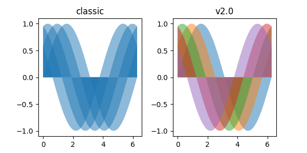
If the facecolor is set via the facecolors or color keyword argument,
then the color is not cycled.
To restore the previous behavior, explicitly pass the keyword argument
facecolors='C0' to the method call.
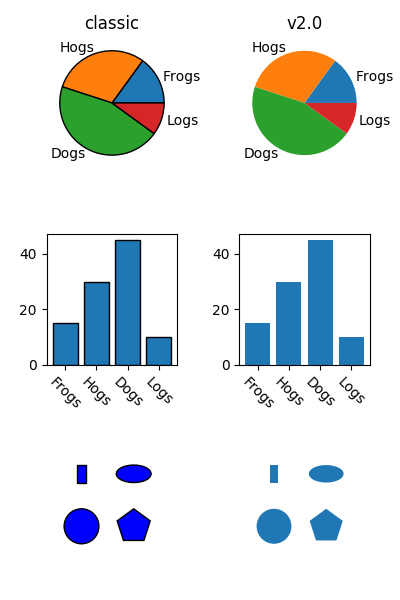
Most artists drawn with a patch (~matplotlib.axes.Axes.bar,
~matplotlib.axes.Axes.pie, etc) no longer have a black edge by
default. The default face color is now 'C0' instead of 'b'.
(Source code, png, pdf)
The previous defaults can be restored by setting:
mpl.rcParams['patch.force_edgecolor'] = True
mpl.rcParams['patch.facecolor'] = 'b'
or by setting:
patch.facecolor        : b
patch.force_edgecolor  : True
in your matplotlibrc file.
hexbin¶The default value of the linecolor kwarg for hexbin has
changed from 'none' to 'face'. If ‘none’ is now supplied, no line edges
are drawn around the hexagons.
bar and barh¶The default value of the align kwarg for both
bar and barh is changed from
'edge' to 'center'.
(Source code, png, pdf)
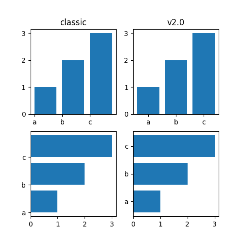
To restore the previous behavior explicitly pass the keyword argument
align='edge' to the method call.
The color of the lines in the hatch is now determined by
- If an edge color is explicitly set, use that for the hatch color
- If the edge color is not explicitly set, use
rcParam['hatch.color']which is looked up at artist creation time.
The width of the lines in a hatch pattern is now configurable by the
rcParams hatch.linewidth, which defaults to 1 point. The old
behavior for the line width was different depending on backend:
- PDF: 0.1 pt
- SVG: 1.0 pt
- PS: 1 px
- Agg: 1 px
The old line width behavior can not be restored across all backends simultaneously, but can be restored for a single backend by setting:
mpl.rcParams['hatch.linewidth'] = 0.1  # previous pdf hatch linewidth
mpl.rcParams['hatch.linewidth'] = 1.0  # previous svg hatch linewidth
The behavior of the PS and Agg backends was DPI dependent, thus:
mpl.rcParams['figure.dpi'] = dpi
mpl.rcParams['savefig.dpi'] = dpi  # or leave as default 'figure'
mpl.rcParams['hatch.linewidth'] = 1.0 / dpi  # previous ps and Agg hatch linewidth
There is no direct API level control of the hatch color or linewidth.
Hatching patterns are now rendered at a consistent density, regardless of DPI. Formerly, high DPI figures would be more dense than the default, and low DPI figures would be less dense. This old behavior cannot be directly restored, but the density may be increased by repeating the hatch specifier.
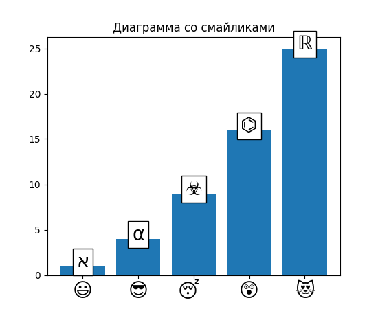
The default font has changed from “Bitstream Vera Sans” to “DejaVu Sans”. DejaVu Sans has additional international and math characters, but otherwise has the same appearance as Bitstream Vera Sans. Latin, Greek, Cyrillic, Armenian, Georgian, Hebrew, and Arabic are all supported (but right-to-left rendering is still not handled by matplotlib). In addition, DejaVu contains a sub-set of emoji symbols.
(Source code, png, pdf)
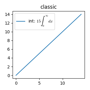
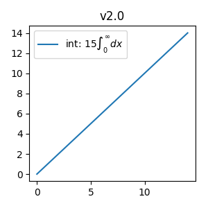
The default math font when using the built-in math rendering engine
(mathtext) has changed from “Computer Modern” (i.e. LaTeX-like) to
“DejaVu Sans”. This change has no effect if the
TeX backend is used (i.e. text.usetex is True).
(Source code, png, pdf)

(Source code, png, pdf)

To revert to the old behavior set the:
mpl.rcParams['mathtext.fontset'] = 'cm'
mpl.rcParams['mathtext.rm'] = 'serif'
or set:
mathtext.fontset: cm
mathtext.rm : serif
in your matplotlibrc file.
This rcParam is consulted when the text is drawn, not when the
artist is created. Thus all mathtext on a given canvas will use the
same fontset.
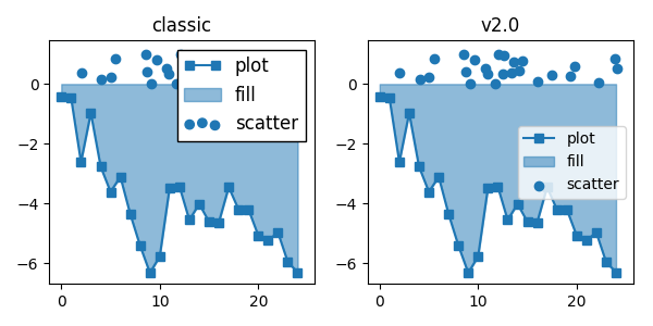
'best', so the legend will be
automatically placed in a location to minimize overlap with data.(Source code, png, pdf)

The previous defaults can be restored by setting:
mpl.rcParams['legend.fancybox'] = False
mpl.rcParams['legend.loc'] = 'upper right'
mpl.rcParams['legend.numpoints'] = 2
mpl.rcParams['legend.fontsize'] = 'large'
mpl.rcParams['legend.framealpha'] = None
mpl.rcParams['legend.scatterpoints'] = 3
mpl.rcParams['legend.edgecolor'] = 'inherit'
or by setting:
legend.fancybox      : False
legend.loc           : upper right
legend.numpoints     : 2      # the number of points in the legend line
legend.fontsize      : large
legend.framealpha    : None    # opacity of legend frame
legend.scatterpoints : 3 # number of scatter points
legend.edgecolor     : inherit   # legend edge color ('inherit'
                                 # means it uses axes.edgecolor)
in your matplotlibrc file.
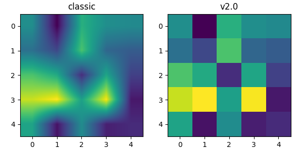
The default interpolation method for imshow is
now 'nearest' and by default it resamples the data (both up and down
sampling) before color mapping.
(Source code, png, pdf)

To restore the previous behavior set:
mpl.rcParams['image.interpolation'] = 'bilinear'
mpl.rcParams['image.resample'] = False
or set:
image.interpolation  : bilinear  # see help(imshow) for options
image.resample  : False
in your matplotlibrc file.
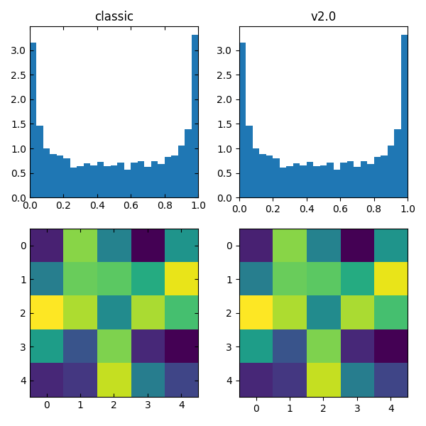
Previously, the input data was normalized, then color mapped, and then resampled to the resolution required for the screen. This meant that the final resampling was being done in color space. Because the color maps are not generally linear in RGB space, colors not in the color map may appear in the final image. This bug was addressed by an almost complete overhaul of the image handling code.
The input data is now normalized, then resampled to the correct resolution (in normalized dataspace), and then color mapped to RGB space. This ensures that only colors from the color map appear in the final image. (If your viewer subsequently resamples the image, the artifact may reappear.)
The previous behavior cannot be restored.
The previous auto-scaling behavior was to find ‘nice’ round numbers as view limits that enclosed the data limits, but this could produce bad plots if the data happened to fall on a vertical or horizontal line near the chosen ‘round number’ limit. The new default sets the view limits to 5% wider than the data range.
(Source code, png, pdf)
The size of the padding in the x and y directions is controlled by the
'axes.xmargin' and 'axes.ymargin' rcParams respectively. Whether
the view limits should be ‘round numbers’ is controlled by the
'axes.autolimit_mode' rcParam. In the original 'round_number' mode,
the view limits coincide with ticks.
The previous default can be restored by using:
mpl.rcParams['axes.autolimit_mode'] = 'round_numbers'
mpl.rcParams['axes.xmargin'] = 0
mpl.rcParams['axes.ymargin'] = 0
or setting:
axes.autolimit_mode: round_numbers
axes.xmargin: 0
axes.ymargin: 0
in your matplotlibrc file.
rcParams['axes.axisbelow'] = False.To reduce the collision of tick marks with data, the default ticks now point outward by default. In addition, ticks are now drawn only on the bottom and left spines to prevent a porcupine appearance, and for a cleaner separation between subplots.
(Source code, png, pdf)

To restore the previous behavior set:
mpl.rcParams['xtick.direction'] = 'in'
mpl.rcParams['ytick.direction'] = 'in'
mpl.rcParams['xtick.top'] = True
mpl.rcParams['ytick.right'] = True
or set:
xtick.top: True
xtick.direction: in

ytick.right: True
ytick.direction: in
in your matplotlibrc file.
The default Locator used for the x and y axis is
AutoLocator which tries to find, up to some
maximum number, ‘nicely’ spaced ticks. The locator now includes
an algorithm to estimate the maximum number of ticks that will leave
room for the tick labels. By default it also ensures that there are at least
two ticks visible.
(Source code, png, pdf)
There is no way, other than using mpl.style.use('classic'), to restore the
previous behavior as the default. On an axis-by-axis basis you may either
control the existing locator via:
ax.xaxis.get_major_locator().set_params(nbins=9, steps=[1, 2, 5, 10])
or create a new MaxNLocator:
import matplotlib.ticker as mticker
ax.set_major_locator(mticker.MaxNLocator(nbins=9, steps=[1, 2, 5, 10])
The algorithm used by MaxNLocator has been
improved, and this may change the choice of tick locations in some
cases. This also affects AutoLocator, which
uses MaxNLocator internally.
For a log-scaled axis the default locator is the
LogLocator. Previously the maximum number
of ticks was set to 15, and could not be changed. Now there is a
numticks kwarg for setting the maximum to any integer value,
to the string ‘auto’, or to its default value of None which is
equivalent to ‘auto’. With the ‘auto’ setting the maximum number
will be no larger than 9, and will be reduced depending on the
length of the axis in units of the tick font size. As in the
case of the AutoLocator, the heuristic algorithm reduces the
incidence of overlapping tick labels but does not prevent it.
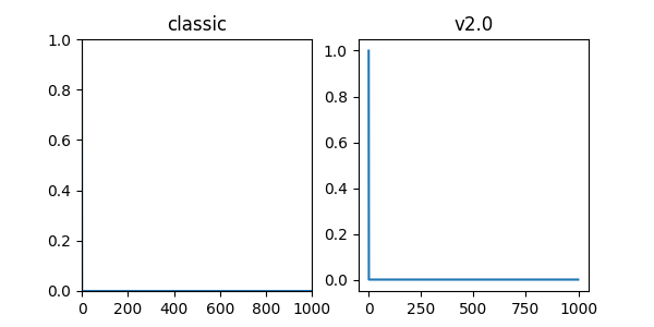
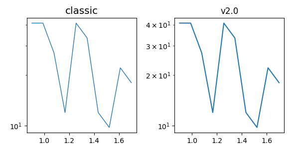
LogFormatter labeling of minor ticks¶Minor ticks on a log axis are now labeled when the axis view limits
span a range less than or equal to the interval between two major
ticks. See LogFormatter for details. The
minor tick labeling is turned off when using mpl.style.use('classic'),
but cannot be controlled independently via rcParams.
(Source code, png, pdf)

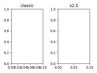
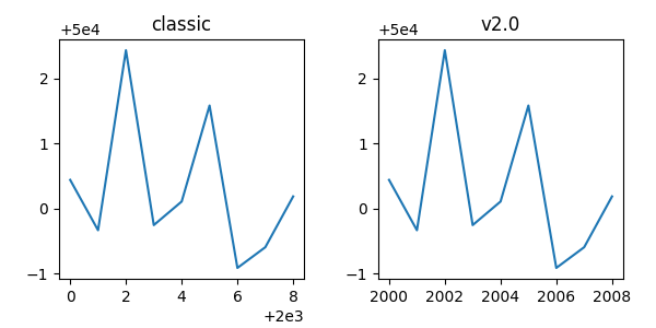
ScalarFormatter tick label formatting with offsets¶With the default of rcParams['axes.formatter.useoffset'] = True,
an offset will be used when it will save 4 or more digits. This can
be controlled with the new rcParam, axes.formatter.offset_threshold.
To restore the previous behavior of using an offset to save 2 or more
digits, use rcParams['axes.formatter.offset_threshold'] = 2.
(Source code, png, pdf)
AutoDateFormatter format strings¶The default date formats are now all based on ISO format, i.e., with
the slowest-moving value first. The date formatters are
configurable through the date.autoformatter.* rcParams.
| Threshold (tick interval >= than) | rcParam | classic | v2.0 |
|---|---|---|---|
| 365 days | 'date.autoformatter.year' |
'%Y' |
'%Y' |
| 30 days | 'date.autoformatter.month' |
'%b %Y' |
'%Y-%m' |
| 1 day | 'date.autoformatter.day' |
'%b %d %Y' |
'%Y-%m-%d' |
| 1 hour | 'date.autoformatter.hour' |
'%H:%M:%S' |
'%H:%M' |
| 1 minute | 'date.autoformatter.minute' |
'%H:%M:%S.%f' |
'%H:%M:%S' |
| 1 second | 'date.autoformatter.second' |
'%H:%M:%S.%f' |
'%H:%M:%S' |
| 1 microsecond | 'date.autoformatter.microsecond' |
'%H:%M:%S.%f' |
'%H:%M:%S.%f' |
Python’s %x and %X date formats may be of particular interest
to format dates based on the current locale.
The previous default can be restored by:
mpl.rcParams['date.autoformatter.year'] = '%Y'
mpl.rcParams['date.autoformatter.month'] = '%b %Y'
mpl.rcParams['date.autoformatter.day'] = '%b %d %Y'
mpl.rcParams['date.autoformatter.hour'] = '%H:%M:%S'
mpl.rcParams['date.autoformatter.minute'] = '%H:%M:%S.%f'
mpl.rcParams['date.autoformatter.second'] = '%H:%M:%S.%f'
mpl.rcParams['date.autoformatter.microsecond'] = '%H:%M:%S.%f'
or setting
date.autoformatter.year   : %Y
date.autoformatter.month  : %b %Y
date.autoformatter.day    : %b %d %Y
date.autoformatter.hour   : %H:%M:%S
date.autoformatter.minute : %H:%M:%S.%f
date.autoformatter.second : %H:%M:%S.%f
date.autoformatter.microsecond : %H:%M:%S.%f
in your matplotlibrc file.