

(Source code, png, pdf)

"""
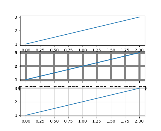
I'm not trying to make a good looking figure here, but just to show
some examples of customizing rc params on the fly
If you like to work interactively, and need to create different sets
of defaults for figures (e.g., one set of defaults for publication, one
set for interactive exploration), you may want to define some
functions in a custom module that set the defaults, e.g.,
def set_pub():
rc('font', weight='bold') # bold fonts are easier to see
rc('tick', labelsize=15) # tick labels bigger
rc('lines', lw=1, color='k') # thicker black lines (no budget for color!)
rc('grid', c='0.5', ls='-', lw=0.5) # solid gray grid lines
rc('savefig', dpi=300) # higher res outputs
Then as you are working interactively, you just need to do
>>> set_pub()
>>> subplot(111)
>>> plot([1,2,3])
>>> savefig('myfig')
>>> rcdefaults() # restore the defaults
"""
import matplotlib.pyplot as plt
plt.subplot(311)
plt.plot([1, 2, 3])
# the axes attributes need to be set before the call to subplot
plt.rc('font', weight='bold')
plt.rc('xtick.major', size=5, pad=7)
plt.rc('xtick', labelsize=15)
# using aliases for color, linestyle and linewidth; gray, solid, thick
plt.rc('grid', c='0.5', ls='-', lw=5)
plt.rc('lines', lw=2, color='g')
plt.subplot(312)
plt.plot([1, 2, 3])
plt.grid(True)
plt.rcdefaults()
plt.subplot(313)
plt.plot([1, 2, 3])
plt.grid(True)
plt.show()
Keywords: python, matplotlib, pylab, example, codex (see Search examples)