

(Source code, png, pdf)
"""
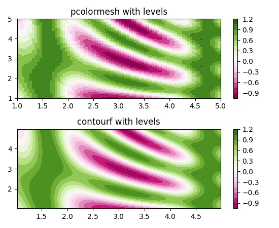
Shows how to combine Normalization and Colormap instances to draw
"levels" in pcolor, pcolormesh and imshow type plots in a similar
way to the levels keyword argument to contour/contourf.
"""
import matplotlib.pyplot as plt
from matplotlib.colors import BoundaryNorm
from matplotlib.ticker import MaxNLocator
import numpy as np
# make these smaller to increase the resolution
dx, dy = 0.05, 0.05
# generate 2 2d grids for the x & y bounds
y, x = np.mgrid[slice(1, 5 + dy, dy),
slice(1, 5 + dx, dx)]
z = np.sin(x)**10 + np.cos(10 + y*x) * np.cos(x)
# x and y are bounds, so z should be the value *inside* those bounds.
# Therefore, remove the last value from the z array.
z = z[:-1, :-1]
levels = MaxNLocator(nbins=15).tick_values(z.min(), z.max())
# pick the desired colormap, sensible levels, and define a normalization
# instance which takes data values and translates those into levels.
cmap = plt.get_cmap('PiYG')
norm = BoundaryNorm(levels, ncolors=cmap.N, clip=True)
fig, (ax0, ax1) = plt.subplots(nrows=2)
im = ax0.pcolormesh(x, y, z, cmap=cmap, norm=norm)
fig.colorbar(im, ax=ax0)
ax0.set_title('pcolormesh with levels')
# contours are *point* based plots, so convert our bound into point
# centers
cf = ax1.contourf(x[:-1, :-1] + dx/2.,
y[:-1, :-1] + dy/2., z, levels=levels,
cmap=cmap)
fig.colorbar(cf, ax=ax1)
ax1.set_title('contourf with levels')
# adjust spacing between subplots so `ax1` title and `ax0` tick labels
# don't overlap
fig.tight_layout()
plt.show()
Keywords: python, matplotlib, pylab, example, codex (see Search examples)