mplot3d example code: surface3d_radial_demo.py

(Source code, png, pdf)

'''
=================================
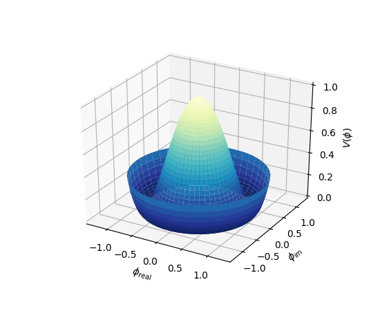
3D surface with polar coordinates
=================================

Demonstrates plotting a surface defined in polar coordinates.
Uses the reversed version of the YlGnBu color map.
Also demonstrates writing axis labels with latex math mode.

Example contributed by Armin Moser.
'''

from mpl_toolkits.mplot3d import Axes3D
from matplotlib import pyplot as plt
import numpy as np


fig = plt.figure()
ax = fig.add_subplot(111, projection='3d')

# Create the mesh in polar coordinates and compute corresponding Z.
r = np.linspace(0, 1.25, 50)
p = np.linspace(0, 2*np.pi, 50)
R, P = np.meshgrid(r, p)
Z = ((R**2 - 1)**2)

# Express the mesh in the cartesian system.
X, Y = R*np.cos(P), R*np.sin(P)

# Plot the surface.
ax.plot_surface(X, Y, Z, cmap=plt.cm.YlGnBu_r)

# Tweak the limits and add latex math labels.
ax.set_zlim(0, 1)
ax.set_xlabel(r'$\phi_\mathrm{real}$')
ax.set_ylabel(r'$\phi_\mathrm{im}$')
ax.set_zlabel(r'$V(\phi)$')

plt.show()

Keywords: python, matplotlib, pylab, example, codex (see Search examples)