

Contents
An Axes3D object is created just like any other axes using
the projection=‘3d’ keyword.
Create a new matplotlib.figure.Figure and
add a new axes to it of type Axes3D:
import matplotlib.pyplot as plt
from mpl_toolkits.mplot3d import Axes3D
fig = plt.figure()
ax = fig.add_subplot(111, projection='3d')
New in version 1.0.0: This approach is the preferred method of creating a 3D axes.
Note
Prior to version 1.0.0, the method of creating a 3D axes was
different. For those using older versions of matplotlib, change
ax = fig.add_subplot(111, projection='3d')
to ax = Axes3D(fig).
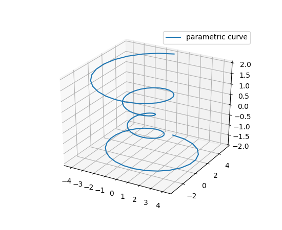
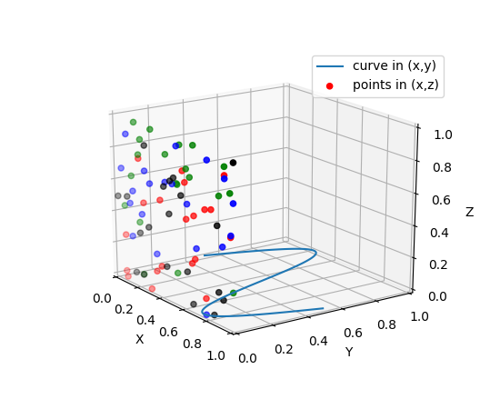
Axes3D.plot(xs, ys, *args, **kwargs)¶Plot 2D or 3D data.
| Argument | Description |
|---|---|
| xs, ys | x, y coordinates of vertices |
| zs | z value(s), either one for all points or one for each point. |
| zdir | Which direction to use as z (‘x’, ‘y’ or ‘z’) when plotting a 2D set. |
Other arguments are passed on to
plot()
(Source code, png, pdf)
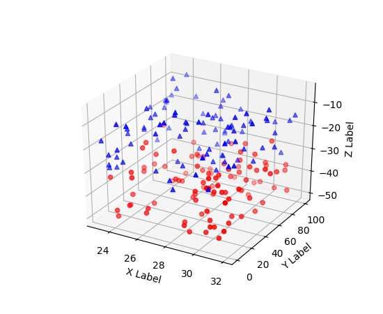
Axes3D.scatter(xs, ys, zs=0, zdir='z', s=20, c=None, depthshade=True, *args, **kwargs)¶Create a scatter plot.
| Argument | Description |
|---|---|
| xs, ys | Positions of data points. |
| zs | Either an array of the same length as xs and ys or a single value to place all points in the same plane. Default is 0. |
| zdir | Which direction to use as z (‘x’, ‘y’ or ‘z’) when plotting a 2D set. |
| s | Size in points^2. It is a scalar or an array of the same length as x and y. |
| c | A color. c can be a single color format string, or a sequence of color specifications of length N, or a sequence of N numbers to be mapped to colors using the cmap and norm specified via kwargs (see below). Note that c should not be a single numeric RGB or RGBA sequence because that is indistinguishable from an array of values to be colormapped. c can be a 2-D array in which the rows are RGB or RGBA, however, including the case of a single row to specify the same color for all points. |
| depthshade | Whether or not to shade the scatter markers to give the appearance of depth. Default is True. |
Keyword arguments are passed on to
scatter().
Returns a Patch3DCollection
(Source code, png, pdf)
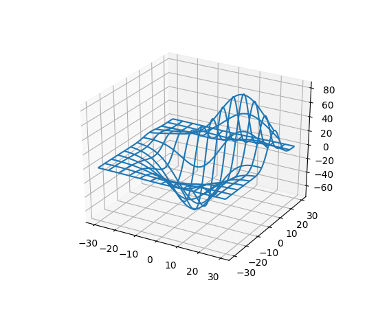
Axes3D.plot_wireframe(X, Y, Z, *args, **kwargs)¶Plot a 3D wireframe.
The
rstrideandcstridekwargs set the stride used to sample the input data to generate the graph. If either is 0 the input data in not sampled along this direction producing a 3D line plot rather than a wireframe plot. The stride arguments are only used by default if in the ‘classic’ mode. They are now superseded byrcountandccount. Will raise ValueError if both stride and count are used.
rcount and ccount kwargs supersedes rstride andcstride for default sampling method for wireframe plotting.
These arguments will determine at most how many evenly spaced
samples will be taken from the input data to generate the graph.
This is the default sampling method unless using the ‘classic’
style. Will raise ValueError if both stride and count are
specified. If either is zero, then the input data is not sampled
along this direction, producing a 3D line plot rather than a
wireframe plot.
Added in v2.0.0.
| Argument | Description |
|---|---|
| X, Y, | Data values as 2D arrays |
| Z | |
| rstride | Array row stride (step size), defaults to 1 |
| cstride | Array column stride (step size), defaults to 1 |
| rcount | Use at most this many rows, defaults to 50 |
| ccount | Use at most this many columns, defaults to 50 |
Keyword arguments are passed on to
LineCollection.
Returns a Line3DCollection
(Source code, png, pdf)

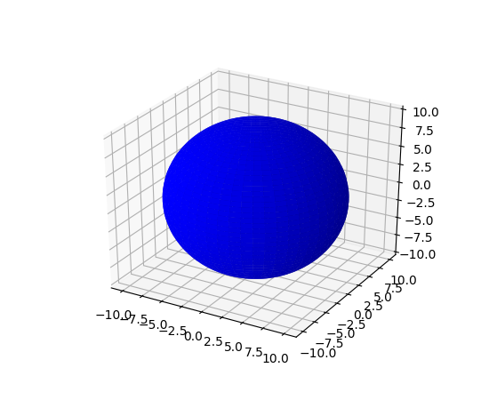
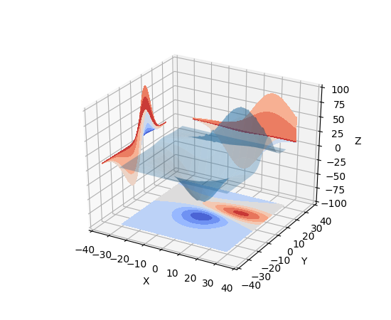
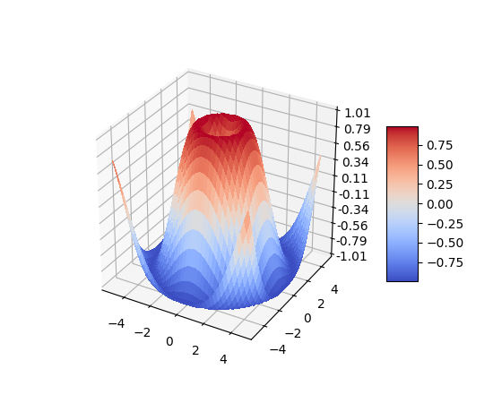
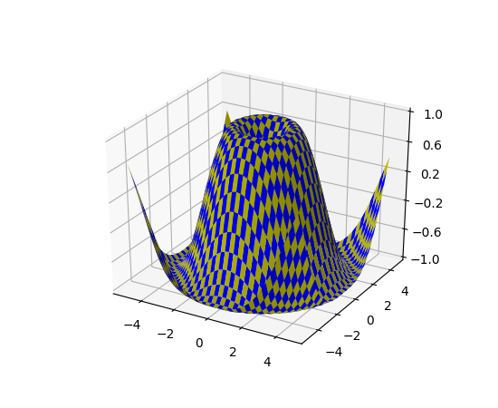
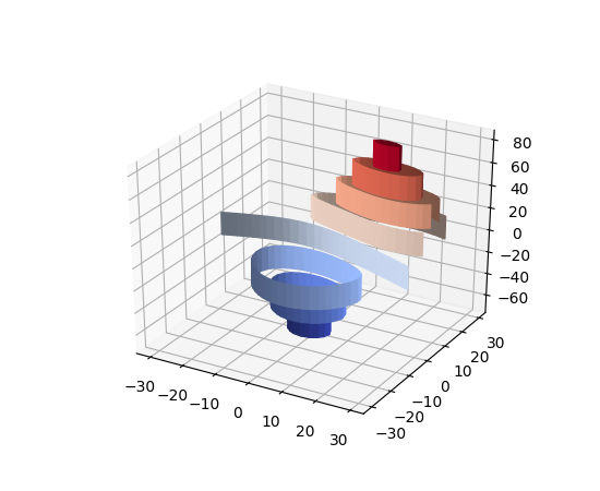
Axes3D.plot_surface(X, Y, Z, *args, **kwargs)¶Create a surface plot.
By default it will be colored in shades of a solid color, but it also supports color mapping by supplying the cmap argument.
The rstride and cstride kwargs set the stride used to
sample the input data to generate the graph. If 1k by 1k
arrays are passed in, the default values for the strides will
result in a 100x100 grid being plotted. Defaults to 10.
Raises a ValueError if both stride and count kwargs
(see next section) are provided.
The rcount and ccount kwargs supersedes rstride and
cstride for default sampling method for surface plotting.
These arguments will determine at most how many evenly spaced
samples will be taken from the input data to generate the graph.
This is the default sampling method unless using the ‘classic’
style. Will raise ValueError if both stride and count are
specified.
Added in v2.0.0.
| Argument | Description |
|---|---|
| X, Y, Z | Data values as 2D arrays |
| rstride | Array row stride (step size) |
| cstride | Array column stride (step size) |
| rcount | Use at most this many rows, defaults to 50 |
| ccount | Use at most this many columns, defaults to 50 |
| color | Color of the surface patches |
| cmap | A colormap for the surface patches. |
| facecolors | Face colors for the individual patches |
| norm | An instance of Normalize to map values to colors |
| vmin | Minimum value to map |
| vmax | Maximum value to map |
| shade | Whether to shade the facecolors |
Other arguments are passed on to
Poly3DCollection
(Source code, png, pdf)

(Source code, png, pdf)
(Source code, png, pdf)

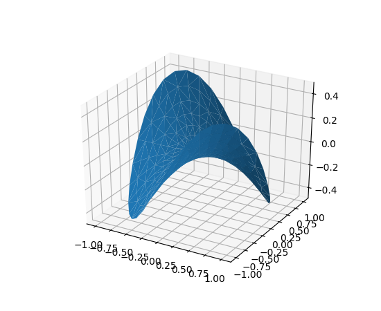
Axes3D.plot_trisurf(*args, **kwargs)¶| Argument | Description |
|---|---|
| X, Y, Z | Data values as 1D arrays |
| color | Color of the surface patches |
| cmap | A colormap for the surface patches. |
| norm | An instance of Normalize to map values to colors |
| vmin | Minimum value to map |
| vmax | Maximum value to map |
| shade | Whether to shade the facecolors |
The (optional) triangulation can be specified in one of two ways; either:
plot_trisurf(triangulation, ...)
where triangulation is a Triangulation
object, or:
plot_trisurf(X, Y, ...)
plot_trisurf(X, Y, triangles, ...)
plot_trisurf(X, Y, triangles=triangles, ...)
in which case a Triangulation object will be created. See
Triangulation for a explanation of
these possibilities.
The remaining arguments are:
plot_trisurf(..., Z)
where Z is the array of values to contour, one per point in the triangulation.
Other arguments are passed on to
Poly3DCollection
Examples:
(Source code, png, pdf)

(Source code, png, pdf)
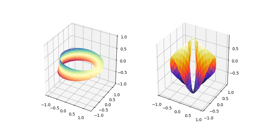
New in version 1.2.0: This plotting function was added for the v1.2.0 release.
(Source code, png, pdf)
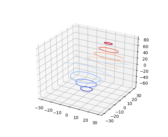
Axes3D.contour(X, Y, Z, *args, **kwargs)¶Create a 3D contour plot.
| Argument | Description |
|---|---|
| X, Y, | Data values as numpy.arrays |
| Z | |
| extend3d | Whether to extend contour in 3D (default: False) |
| stride | Stride (step size) for extending contour |
| zdir | The direction to use: x, y or z (default) |
| offset | If specified plot a projection of the contour lines on this position in plane normal to zdir |
The positional and other keyword arguments are passed on to
contour()
Returns a contour
(Source code, png, pdf)
(Source code, png, pdf)

(Source code, png, pdf)

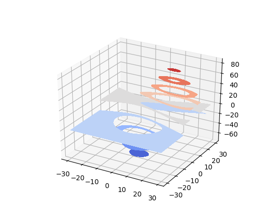
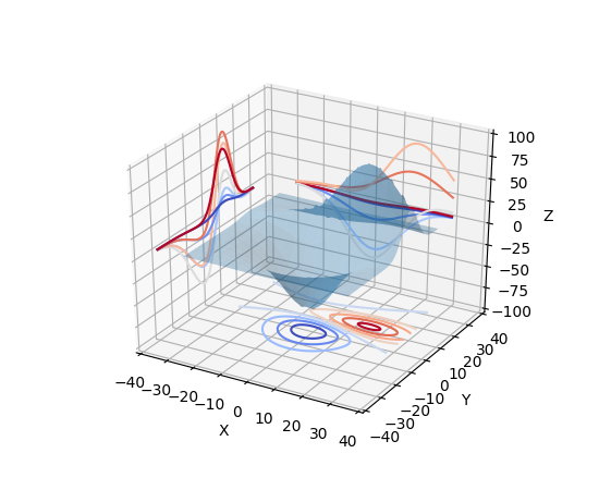
Axes3D.contourf(X, Y, Z, *args, **kwargs)¶Create a 3D contourf plot.
| Argument | Description |
|---|---|
| X, Y, | Data values as numpy.arrays |
| Z | |
| zdir | The direction to use: x, y or z (default) |
| offset | If specified plot a projection of the filled contour on this position in plane normal to zdir |
The positional and keyword arguments are passed on to
contourf()
Returns a contourf
Changed in version 1.1.0: The zdir and offset kwargs were added.
(Source code, png, pdf)
(Source code, png, pdf)
New in version 1.1.0: The feature demoed in the second contourf3d example was enabled as a result of a bugfix for version 1.1.0.
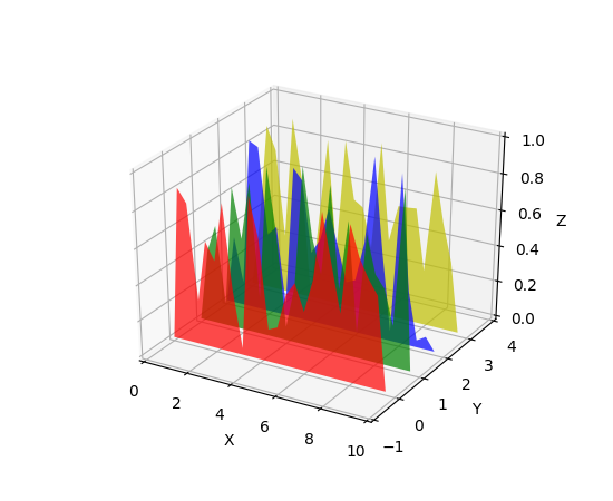
Axes3D.add_collection3d(col, zs=0, zdir='z')¶Add a 3D collection object to the plot.
2D collection types are converted to a 3D version by modifying the object and adding z coordinate information.
(Source code, png, pdf)

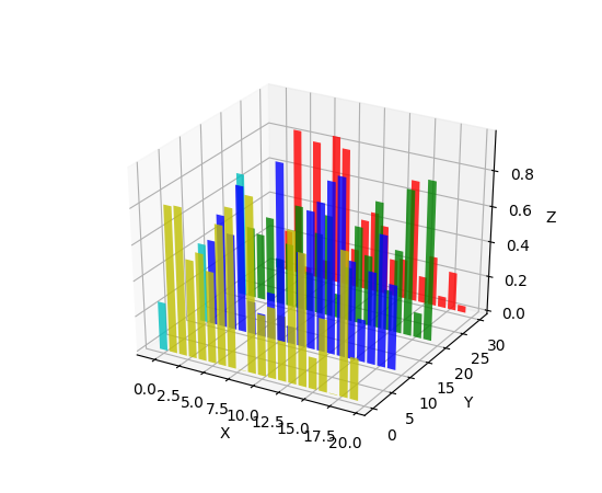
Axes3D.bar(left, height, zs=0, zdir='z', *args, **kwargs)¶Add 2D bar(s).
| Argument | Description |
|---|---|
| left | The x coordinates of the left sides of the bars. |
| height | The height of the bars. |
| zs | Z coordinate of bars, if one value is specified they will all be placed at the same z. |
| zdir | Which direction to use as z (‘x’, ‘y’ or ‘z’) when plotting a 2D set. |
Keyword arguments are passed onto bar().
Returns a Patch3DCollection
(Source code, png, pdf)
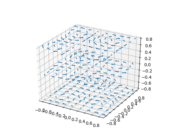
Axes3D.quiver(*args, **kwargs)¶Plot a 3D field of arrows.
call signatures:
quiver(X, Y, Z, U, V, W, **kwargs)
Arguments:
- X, Y, Z:
- The x, y and z coordinates of the arrow locations (default is tail of arrow; see pivot kwarg)
- U, V, W:
- The x, y and z components of the arrow vectors
The arguments could be array-like or scalars, so long as they they can be broadcast together. The arguments can also be masked arrays. If an element in any of argument is masked, then that corresponding quiver element will not be plotted.
Keyword arguments:
- length: [1.0 | float]
- The length of each quiver, default to 1.0, the unit is the same with the axes
- arrow_length_ratio: [0.3 | float]
- The ratio of the arrow head with respect to the quiver, default to 0.3
- pivot: [ ‘tail’ | ‘middle’ | ‘tip’ ]
- The part of the arrow that is at the grid point; the arrow rotates about this point, hence the name pivot. Default is ‘tail’
- normalize: [False | True]
- When True, all of the arrows will be the same length. This defaults to False, where the arrows will be different lengths depending on the values of u,v,w.
Any additional keyword arguments are delegated to
LineCollection
(Source code, png, pdf)
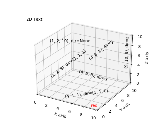
Axes3D.text(x, y, z, s, zdir=None, **kwargs)¶Add text to the plot. kwargs will be passed on to Axes.text,
except for the zdir keyword, which sets the direction to be
used as the z direction.
(Source code, png, pdf)

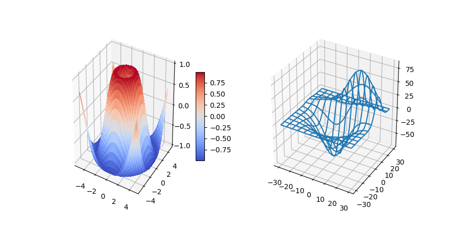
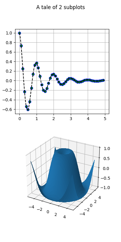
Having multiple 3D plots in a single figure is the same as it is for 2D plots. Also, you can have both 2D and 3D plots in the same figure.
New in version 1.0.0: Subplotting 3D plots was added in v1.0.0. Earlier version can not do this.
(Source code, png, pdf)
(Source code, png, pdf)