You are reading an old version of the documentation (v2.0.0). For the latest version see https://matplotlib.org/stable/api/_as_gen/matplotlib.axes.Axes.psd.html
matplotlib

Travis-CI:

This Page

matplotlib.axes.Axes.psd

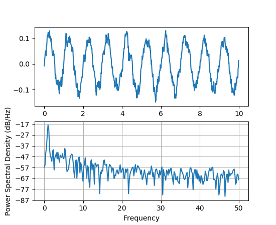
Axes.psd(x, NFFT=None, Fs=None, Fc=None, detrend=None, window=None, noverlap=None, pad_to=None, sides=None, scale_by_freq=None, return_line=None, **kwargs)

Plot the power spectral density.

Call signature:

psd(x, NFFT=256, Fs=2, Fc=0, detrend=mlab.detrend_none,
    window=mlab.window_hanning, noverlap=0, pad_to=None,
    sides='default', scale_by_freq=None, return_line=None, **kwargs)

The power spectral density by Welch’s average periodogram method. The vector x is divided into NFFT length segments. Each segment is detrended by function detrend and windowed by function window. noverlap gives the length of the overlap between segments. The of each segment are averaged to compute , with a scaling to correct for power loss due to windowing.

If len(x) < NFFT, it will be zero padded to NFFT.

Parameters:

x : 1-D array or sequence

Array or sequence containing the data

Fs : scalar

The sampling frequency (samples per time unit). It is used to calculate the Fourier frequencies, freqs, in cycles per time unit. The default value is 2.

window : callable or ndarray

A function or a vector of length NFFT. To create window vectors see window_hanning(), window_none(), numpy.blackman(), numpy.hamming(), numpy.bartlett(), scipy.signal(), scipy.signal.get_window(), etc. The default is window_hanning(). If a function is passed as the argument, it must take a data segment as an argument and return the windowed version of the segment.

sides : [ ‘default’ | ‘onesided’ | ‘twosided’ ]

Specifies which sides of the spectrum to return. Default gives the default behavior, which returns one-sided for real data and both for complex data. ‘onesided’ forces the return of a one-sided spectrum, while ‘twosided’ forces two-sided.

pad_to : integer

The number of points to which the data segment is padded when performing the FFT. This can be different from NFFT, which specifies the number of data points used. While not increasing the actual resolution of the spectrum (the minimum distance between resolvable peaks), this can give more points in the plot, allowing for more detail. This corresponds to the n parameter in the call to fft(). The default is None, which sets pad_to equal to NFFT

NFFT : integer

The number of data points used in each block for the FFT. A power 2 is most efficient. The default value is 256. This should NOT be used to get zero padding, or the scaling of the result will be incorrect. Use pad_to for this instead.

detrend : {‘default’, ‘constant’, ‘mean’, ‘linear’, ‘none’} or callable

The function applied to each segment before fft-ing, designed to remove the mean or linear trend. Unlike in MATLAB, where the detrend parameter is a vector, in matplotlib is it a function. The pylab module defines detrend_none(), detrend_mean(), and detrend_linear(), but you can use a custom function as well. You can also use a string to choose one of the functions. ‘default’, ‘constant’, and ‘mean’ call detrend_mean(). ‘linear’ calls detrend_linear(). ‘none’ calls detrend_none().

scale_by_freq : boolean, optional

Specifies whether the resulting density values should be scaled by the scaling frequency, which gives density in units of Hz^-1. This allows for integration over the returned frequency values. The default is True for MATLAB compatibility.

noverlap : integer

The number of points of overlap between segments. The default value is 0 (no overlap).

Fc : integer

The center frequency of x (defaults to 0), which offsets the x extents of the plot to reflect the frequency range used when a signal is acquired and then filtered and downsampled to baseband.

return_line : bool

Whether to include the line object plotted in the returned values. Default is False.

**kwargs :

Keyword arguments control the Line2D properties:

Property Description
agg_filter unknown
alpha float (0.0 transparent through 1.0 opaque)
animated [True | False]
antialiased or aa [True | False]
axes an Axes instance
clip_box a matplotlib.transforms.Bbox instance
clip_on [True | False]
clip_path [ (Path, Transform) | Patch | None ]
color or c any matplotlib color
contains a callable function
dash_capstyle [‘butt’ | ‘round’ | ‘projecting’]
dash_joinstyle [‘miter’ | ‘round’ | ‘bevel’]
dashes sequence of on/off ink in points
drawstyle [‘default’ | ‘steps’ | ‘steps-pre’ | ‘steps-mid’ | ‘steps-post’]
figure a matplotlib.figure.Figure instance
fillstyle [‘full’ | ‘left’ | ‘right’ | ‘bottom’ | ‘top’ | ‘none’]
gid an id string
label string or anything printable with ‘%s’ conversion.
linestyle or ls [‘solid’ | ‘dashed’, ‘dashdot’, ‘dotted’ | (offset, on-off-dash-seq) | '-' | '--' | '-.' | ':' | 'None' | ' ' | '']
linewidth or lw float value in points
marker A valid marker style
markeredgecolor or mec any matplotlib color
markeredgewidth or mew float value in points
markerfacecolor or mfc any matplotlib color
markerfacecoloralt or mfcalt any matplotlib color
markersize or ms float
markevery [None | int | length-2 tuple of int | slice | list/array of int | float | length-2 tuple of float]
path_effects unknown
picker float distance in points or callable pick function fn(artist, event)
pickradius float distance in points
rasterized [True | False | None]
sketch_params unknown
snap unknown
solid_capstyle [‘butt’ | ‘round’ | ‘projecting’]
solid_joinstyle [‘miter’ | ‘round’ | ‘bevel’]
transform a matplotlib.transforms.Transform instance
url a url string
visible [True | False]
xdata 1D array
ydata 1D array
zorder any number
Returns:

Pxx : 1-D array

The values for the power spectrum P_{xx} before scaling (real valued)

freqs : 1-D array

The frequencies corresponding to the elements in Pxx

line : a Line2D instance

The line created by this function. Only returned if return_line is True.

See also

specgram()
specgram() differs in the default overlap; in not returning the mean of the segment periodograms; in returning the times of the segments; and in plotting a colormap instead of a line.
magnitude_spectrum()
magnitude_spectrum() plots the magnitude spectrum.
csd()
csd() plots the spectral density between two signals.
In addition to the above described arguments, this function can take a data keyword argument. If such a data argument is given, the following arguments are replaced by data[<arg>]: * All arguments with the following names: ‘x’.

Notes

For plotting, the power is plotted as for decibels, though Pxx itself is returned.

References

Bendat & Piersol – Random Data: Analysis and Measurement Procedures, John Wiley & Sons (1986)

Examples

(Source code, png, pdf)

../../_images/psd_demo_00_00.png