Learn what to expect in the new updates


For a more detailed introduction to annotations, see Annotating Axes.
The uses of the basic text() command above
place text at an arbitrary position on the Axes. A common use case of
text is to annotate some feature of the plot, and the
annotate() method provides helper functionality
to make annotations easy. In an annotation, there are two points to
consider: the location being annotated represented by the argument
xy and the location of the text xytext. Both of these
arguments are (x,y) tuples.
import numpy as np
import matplotlib.pyplot as plt

fig = plt.figure()
ax = fig.add_subplot(111)

t = np.arange(0.0, 5.0, 0.01)
s = np.cos(2*np.pi*t)
line, = ax.plot(t, s, lw=2)

ax.annotate('local max', xy=(2, 1), xytext=(3, 1.5),
            arrowprops=dict(facecolor='black', shrink=0.05),
            )

ax.set_ylim(-2,2)
plt.show()
(Source code, png, hires.png, pdf)
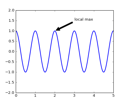
In this example, both the xy (arrow tip) and xytext locations
(text location) are in data coordinates. There are a variety of other
coordinate systems one can choose – you can specify the coordinate
system of xy and xytext with one of the following strings for
xycoords and textcoords (default is ‘data’)
| argument | coordinate system |
|---|---|
| ‘figure points’ | points from the lower left corner of the figure |
| ‘figure pixels’ | pixels from the lower left corner of the figure |
| ‘figure fraction’ | 0,0 is lower left of figure and 1,1 is upper right |
| ‘axes points’ | points from lower left corner of axes |
| ‘axes pixels’ | pixels from lower left corner of axes |
| ‘axes fraction’ | 0,0 is lower left of axes and 1,1 is upper right |
| ‘data’ | use the axes data coordinate system |
For example to place the text coordinates in fractional axes coordinates, one could do:
ax.annotate('local max', xy=(3, 1),  xycoords='data',
            xytext=(0.8, 0.95), textcoords='axes fraction',
            arrowprops=dict(facecolor='black', shrink=0.05),
            horizontalalignment='right', verticalalignment='top',
            )
For physical coordinate systems (points or pixels) the origin is the (bottom, left) of the figure or axes. If the value is negative, however, the origin is from the (right, top) of the figure or axes, analogous to negative indexing of sequences.
Optionally, you can specify arrow properties which draws an arrow
from the text to the annotated point by giving a dictionary of arrow
properties in the optional keyword argument arrowprops.
arrowprops key |
description |
|---|---|
| width | the width of the arrow in points |
| frac | the fraction of the arrow length occupied by the head |
| headwidth | the width of the base of the arrow head in points |
| shrink | move the tip and base some percent away from the annotated point and text |
| **kwargs | any key for matplotlib.patches.Polygon,
e.g., facecolor |
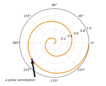
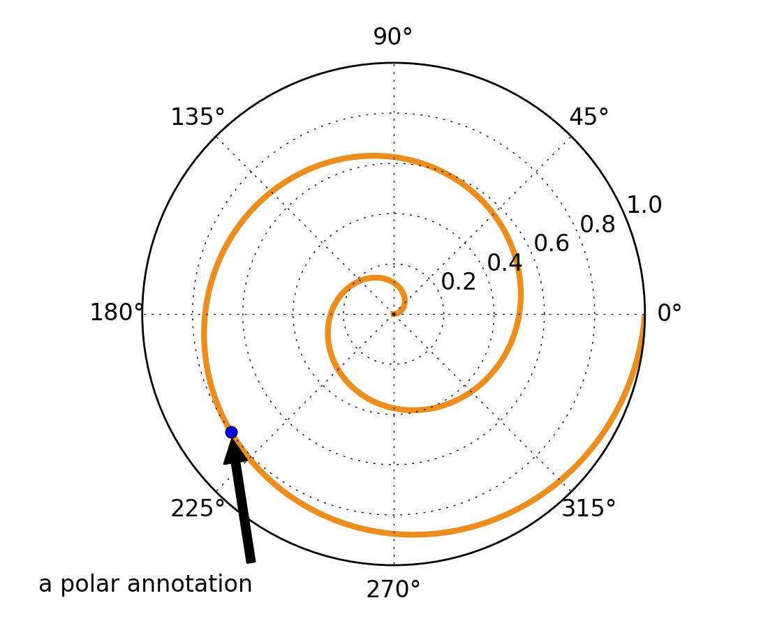
In the example below, the xy point is in native coordinates
(xycoords defaults to ‘data’). For a polar axes, this is in
(theta, radius) space. The text in this example is placed in the
fractional figure coordinate system. matplotlib.text.Text
keyword args like horizontalalignment, verticalalignment and
fontsize are passed from the `~matplotlib.Axes.annotate` to the
``Text
instance
import numpy as np
import matplotlib.pyplot as plt

fig = plt.figure()
ax = fig.add_subplot(111, polar=True)
r = np.arange(0,1,0.001)
theta = 2*2*np.pi*r
line, = ax.plot(theta, r, color='#ee8d18', lw=3)

ind = 800
thisr, thistheta = r[ind], theta[ind]
ax.plot([thistheta], [thisr], 'o')
ax.annotate('a polar annotation',
            xy=(thistheta, thisr),  # theta, radius
            xytext=(0.05, 0.05),    # fraction, fraction
            textcoords='figure fraction',
            arrowprops=dict(facecolor='black', shrink=0.05),
            horizontalalignment='left',
            verticalalignment='bottom',
            )
plt.show()
(Source code, png, hires.png, pdf)
For more on all the wild and wonderful things you can do with annotations, including fancy arrows, see Annotating Axes and pylab_examples example code: annotation_demo.py.