Learn what to expect in the new updates


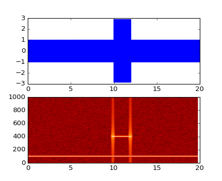
(Source code, png, hires.png, pdf)

import matplotlib.pyplot as plt
import numpy as np

dt = 0.0005
t = np.arange(0.0, 20.0, dt)
s1 = np.sin(2*np.pi*100*t)
s2 = 2*np.sin(2*np.pi*400*t)

# create a transient "chirp"
mask = np.where(np.logical_and(t > 10, t < 12), 1.0, 0.0)
s2 = s2 * mask

# add some noise into the mix
nse = 0.01*np.random.random(size=len(t))

x = s1 + s2 + nse  # the signal
NFFT = 1024       # the length of the windowing segments
Fs = int(1.0/dt)  # the sampling frequency

# Pxx is the segments x freqs array of instantaneous power, freqs is
# the frequency vector, bins are the centers of the time bins in which
# the power is computed, and im is the matplotlib.image.AxesImage
# instance

ax1 = plt.subplot(211)
plt.plot(t, x)
plt.subplot(212, sharex=ax1)
Pxx, freqs, bins, im = plt.specgram(x, NFFT=NFFT, Fs=Fs, noverlap=900,
                                cmap=plt.cm.gist_heat)
plt.show()
Keywords: python, matplotlib, pylab, example, codex (see Search examples)