Learn what to expect in the new updates

tight_layout automatically adjusts subplot params so that the subplot(s) fits in to the figure area. This is an experimental feature and may not work for some cases. It only checks the extents of ticklabels, axis labels, and titles.
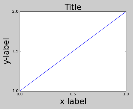
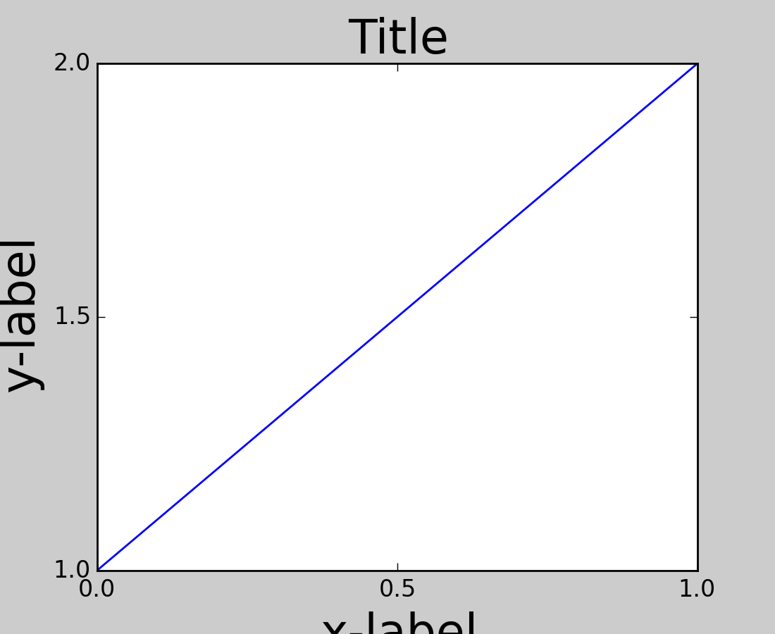
In matplotlib, the location of axes (including subplots) are specified in normalized figure coordinates. It can happen that your axis labels or titles (or sometimes even ticklabels) go outside the figure area, and are thus clipped.
plt.rcParams['savefig.facecolor'] = "0.8"
def example_plot(ax, fontsize=12):
ax.plot([1, 2])
ax.locator_params(nbins=3)
ax.set_xlabel('x-label', fontsize=fontsize)
ax.set_ylabel('y-label', fontsize=fontsize)
ax.set_title('Title', fontsize=fontsize)
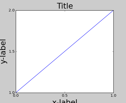
plt.close('all')
fig, ax = plt.subplots()
example_plot(ax, fontsize=24)
(Source code, png, hires.png, pdf)

To prevent this, the location of axes needs to be adjusted. For subplots, this can be done by adjusting the subplot params (Move the edge of an axes to make room for tick labels). Matplotlib v1.1 introduces a new command tight_layout() that does this automatically for you.
plt.tight_layout()
(Source code, png, hires.png, pdf)
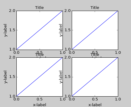
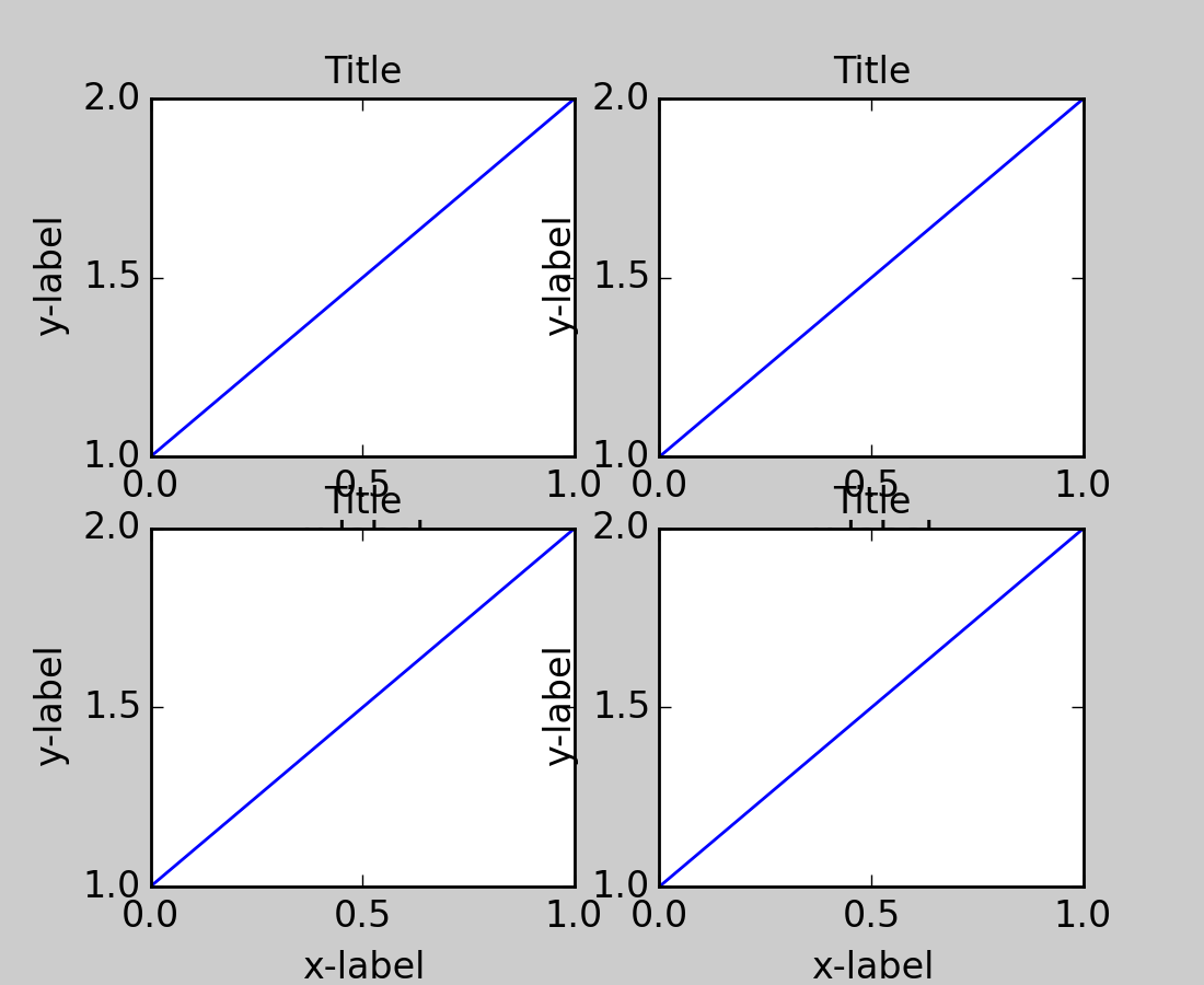
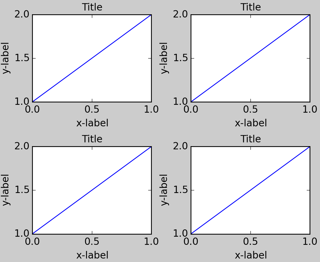
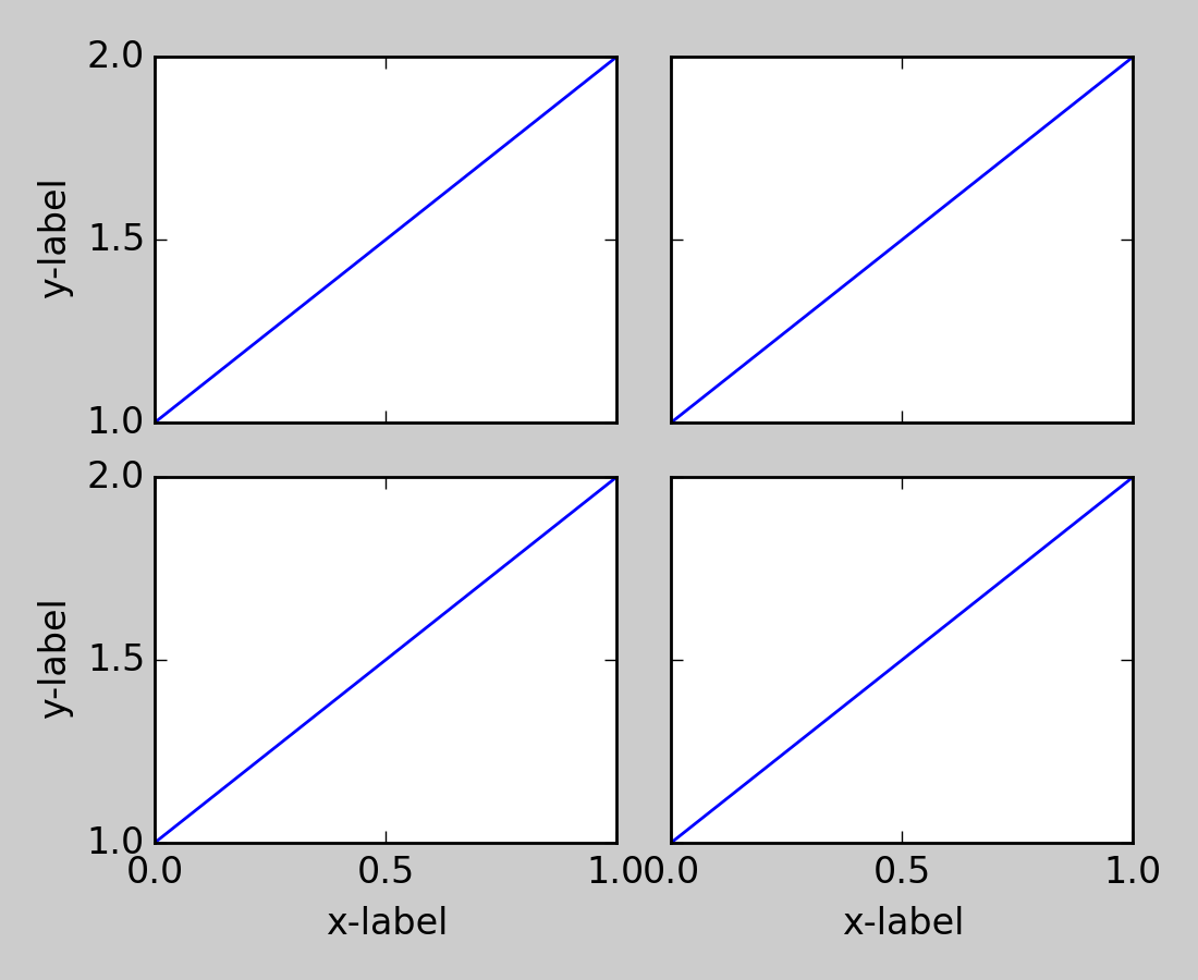
When you have multiple subplots, often you see labels of different axes overlapping each other.
plt.close('all')
fig, ((ax1, ax2), (ax3, ax4)) = plt.subplots(nrows=2, ncols=2)
example_plot(ax1)
example_plot(ax2)
example_plot(ax3)
example_plot(ax4)
(Source code, png, hires.png, pdf)
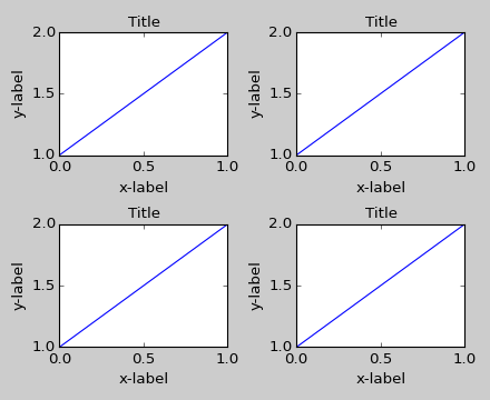
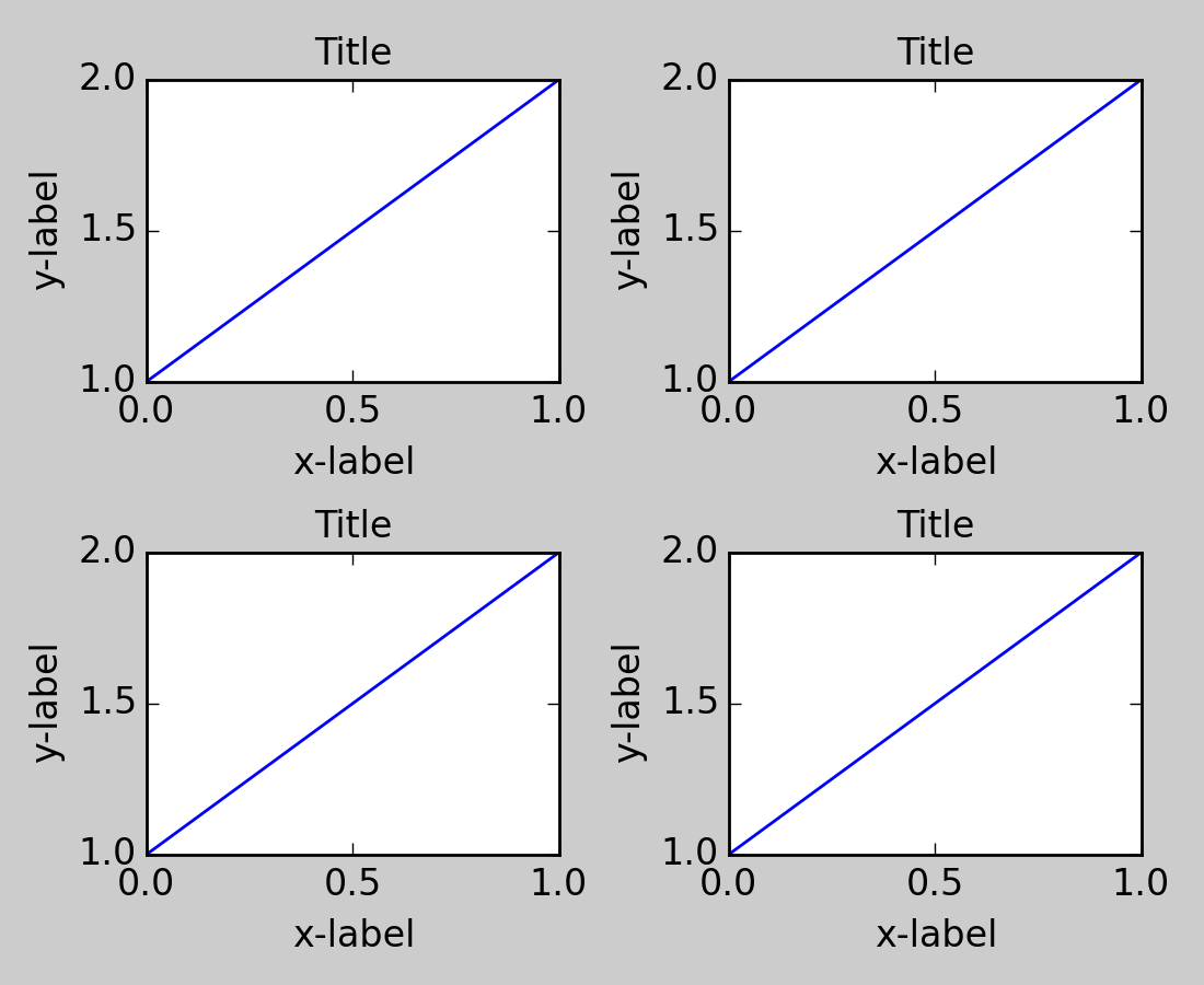
tight_layout() will also adjust spacing between subplots to minimize the overlaps.
plt.tight_layout()
(Source code, png, hires.png, pdf)
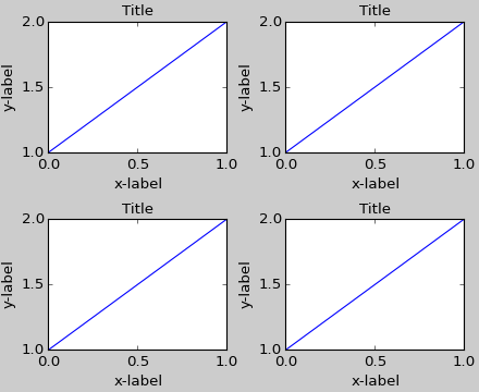
tight_layout() can take keyword arguments of pad, w_pad and h_pad. These control the extra padding around the figure border and between subplots. The pads are specified in fraction of fontsize.
plt.tight_layout(pad=0.4, w_pad=0.5, h_pad=1.0)
(Source code, png, hires.png, pdf)

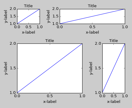
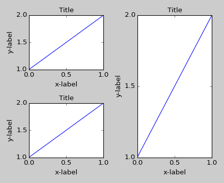
tight_layout() will work even if the sizes of subplots are different as far as their grid specification is compatible. In the example below, ax1 and ax2 are subplots of a 2x2 grid, while ax3 is of a 1x2 grid.
plt.close('all')
fig = plt.figure()

ax1 = plt.subplot(221)
ax2 = plt.subplot(223)
ax3 = plt.subplot(122)

example_plot(ax1)
example_plot(ax2)
example_plot(ax3)

plt.tight_layout()
(Source code, png, hires.png, pdf)

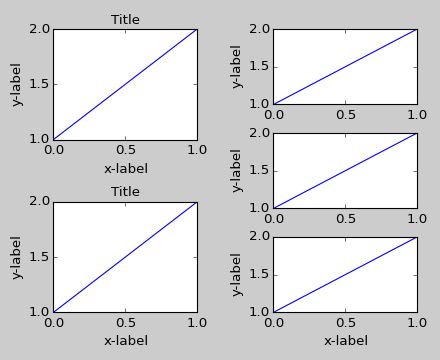
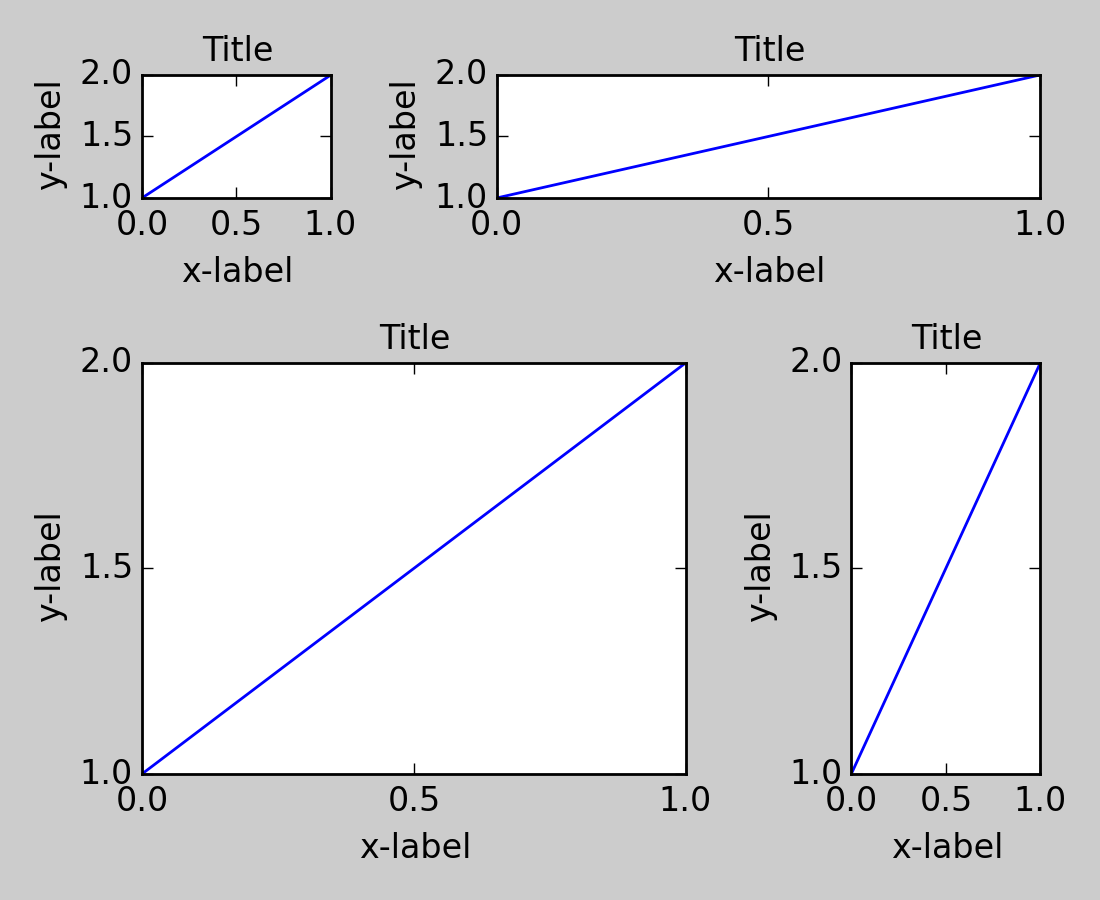
It works with subplots created with subplot2grid(). In general, subplots created from the gridspec (Customizing Location of Subplot Using GridSpec) will work.
plt.close('all')
fig = plt.figure()

ax1 = plt.subplot2grid((3, 3), (0, 0))
ax2 = plt.subplot2grid((3, 3), (0, 1), colspan=2)
ax3 = plt.subplot2grid((3, 3), (1, 0), colspan=2, rowspan=2)
ax4 = plt.subplot2grid((3, 3), (1, 2), rowspan=2)

example_plot(ax1)
example_plot(ax2)
example_plot(ax3)
example_plot(ax4)

plt.tight_layout()
(Source code, png, hires.png, pdf)
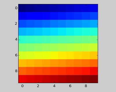
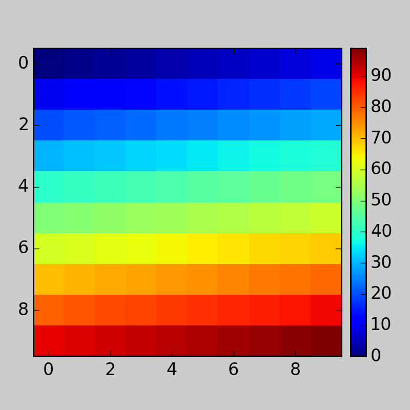
Although not thoroughly tested, it seems to work for subplots with aspect != “auto” (e.g., axes with images).
arr = np.arange(100).reshape((10,10))

plt.close('all')
fig = plt.figure(figsize=(5,4))

ax = plt.subplot(111)
im = ax.imshow(arr, interpolation="none")

plt.tight_layout()
(Source code, png, hires.png, pdf)

- tight_layout() only considers ticklabels, axis labels, and titles. Thus, other artists may be clipped and also may overlap.
- It assumes that the extra space needed for ticklabels, axis labels, and titles is independent of original location of axes. This is often true, but there are rare cases where it is not.
- pad=0 clips some of the texts by a few pixels. This may be a bug or a limitation of the current algorithm and it is not clear why it happens. Meanwhile, use of pad at least larger than 0.3 is recommended.
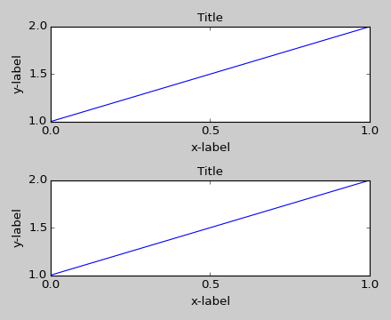
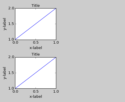
GridSpec has its own tight_layout() method (the pyplot api tight_layout() also works).
plt.close('all')
fig = plt.figure()

import matplotlib.gridspec as gridspec

gs1 = gridspec.GridSpec(2, 1)
ax1 = fig.add_subplot(gs1[0])
ax2 = fig.add_subplot(gs1[1])

example_plot(ax1)
example_plot(ax2)

gs1.tight_layout(fig)
(Source code, png, hires.png, pdf)
You may provide an optional rect parameter, which specifies the bounding box that the subplots will be fit inside. The coordinates must be in normalized figure coordinates and the default is (0, 0, 1, 1).
gs1.tight_layout(fig, rect=[0, 0, 0.5, 1])
(Source code, png, hires.png, pdf)

For example, this can be used for a figure with multiple gridspecs.
gs2 = gridspec.GridSpec(3, 1)

for ss in gs2:
    ax = fig.add_subplot(ss)
    example_plot(ax)
    ax.set_title("")
    ax.set_xlabel("")

ax.set_xlabel("x-label", fontsize=12)

gs2.tight_layout(fig, rect=[0.5, 0, 1, 1], h_pad=0.5)
(Source code, png, hires.png, pdf)

We may try to match the top and bottom of two grids
top = min(gs1.top, gs2.top)
bottom = max(gs1.bottom, gs2.bottom)

gs1.update(top=top, bottom=bottom)
gs2.update(top=top, bottom=bottom)
While this should be mostly good enough, adjusting top and bottom may require adjustment of hspace also. To update hspace & vspace, we call tight_layout() again with updated rect argument. Note that the rect argument specifies the area including the ticklabels, etc. Thus, we will increase the bottom (which is 0 for the normal case) by the difference between the bottom from above and the bottom of each gridspec. Same thing for the top.
top = min(gs1.top, gs2.top)
bottom = max(gs1.bottom, gs2.bottom)

gs1.tight_layout(fig, rect=[None, 0 + (bottom-gs1.bottom),
                            0.5, 1 - (gs1.top-top)])
gs2.tight_layout(fig, rect=[0.5, 0 + (bottom-gs2.bottom),
                            None, 1 - (gs2.top-top)],
                 h_pad=0.5)
(Source code, png, hires.png, pdf)
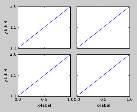
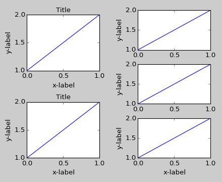
While limited, the axes_grid1 toolkit is also supported.
plt.close('all')
fig = plt.figure()

from mpl_toolkits.axes_grid1 import Grid
grid = Grid(fig, rect=111, nrows_ncols=(2,2),
            axes_pad=0.25, label_mode='L',
            )

for ax in grid:
    example_plot(ax)
    ax.title.set_visible(False)

plt.tight_layout()
(Source code, png, hires.png, pdf)
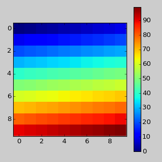
If you create a colorbar with the colorbar() command, the created colorbar is an instance of Axes, not Subplot, so tight_layout does not work. With Matplotlib v1.1, you may create a colorbar as a subplot using the gridspec.
plt.close('all')
fig = plt.figure(figsize=(4, 4))
im = plt.imshow(arr, interpolation="none")

plt.colorbar(im, use_gridspec=True)

plt.tight_layout()
(Source code, png, hires.png, pdf)

Another option is to use AxesGrid1 toolkit to explicitly create an axes for colorbar.
plt.close('all')
fig = plt.figure(figsize=(4, 4))
im = plt.imshow(arr, interpolation="none")

from mpl_toolkits.axes_grid1 import make_axes_locatable
divider = make_axes_locatable(plt.gca())
cax = divider.append_axes("right", "5%", pad="3%")
plt.colorbar(im, cax=cax)

plt.tight_layout()
(Source code, png, hires.png, pdf)
