
"""
Some examples of how to annotate points in figures. You specify an
annotation point xy=(x,y) and a text point xytext=(x,y) for the
annotated points and text location, respectively. Optionally, you can
specify the coordinate system of xy and xytext with one of the
following strings for xycoords and textcoords (default is 'data')
'figure points' : points from the lower left corner of the figure
'figure pixels' : pixels from the lower left corner of the figure
'figure fraction' : 0,0 is lower left of figure and 1,1 is upper, right
'axes points' : points from lower left corner of axes
'axes pixels' : pixels from lower left corner of axes
'axes fraction' : 0,0 is lower left of axes and 1,1 is upper right
'offset points' : Specify an offset (in points) from the xy value
'data' : use the axes data coordinate system
Optionally, you can specify arrow properties which draws and arrow
from the text to the annotated point by giving a dictionary of arrow
properties
Valid keys are
width : the width of the arrow in points
frac : the fraction of the arrow length occupied by the head
headwidth : the width of the base of the arrow head in points
shrink : move the tip and base some percent away from the
annotated point and text
any key for matplotlib.patches.polygon (eg facecolor)
For physical coordinate systems (points or pixels) the origin is the
(bottom, left) of the figure or axes. If the value is negative,
however, the origin is from the (right, top) of the figure or axes,
analogous to negative indexing of sequences.
"""
from matplotlib.pyplot import figure, show
from matplotlib.patches import Ellipse
import numpy as np
if 1:
# if only one location is given, the text and xypoint being
# annotated are assumed to be the same
fig = figure()
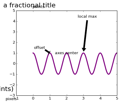
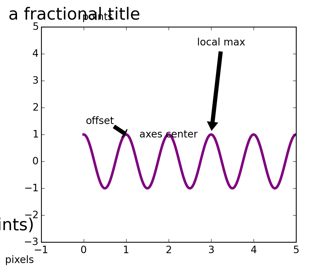
ax = fig.add_subplot(111, autoscale_on=False, xlim=(-1,5), ylim=(-3,5))
t = np.arange(0.0, 5.0, 0.01)
s = np.cos(2*np.pi*t)
line, = ax.plot(t, s, lw=3, color='purple')
ax.annotate('axes center', xy=(.5, .5), xycoords='axes fraction',
horizontalalignment='center', verticalalignment='center')
ax.annotate('pixels', xy=(20, 20), xycoords='figure pixels')
ax.annotate('points', xy=(100, 300), xycoords='figure points')
ax.annotate('offset', xy=(1, 1), xycoords='data',
xytext=(-15, 10), textcoords='offset points',
arrowprops=dict(facecolor='black', shrink=0.05),
horizontalalignment='right', verticalalignment='bottom',
)
ax.annotate('local max', xy=(3, 1), xycoords='data',
xytext=(0.8, 0.95), textcoords='axes fraction',
arrowprops=dict(facecolor='black', shrink=0.05),
horizontalalignment='right', verticalalignment='top',
)
ax.annotate('a fractional title', xy=(.025, .975),
xycoords='figure fraction',
horizontalalignment='left', verticalalignment='top',
fontsize=20)
# use negative points or pixels to specify from right, top -10, 10
# is 10 points to the left of the right side of the axes and 10
# points above the bottom
ax.annotate('bottom right (points)', xy=(-10, 10),
xycoords='axes points',
horizontalalignment='right', verticalalignment='bottom',
fontsize=20)
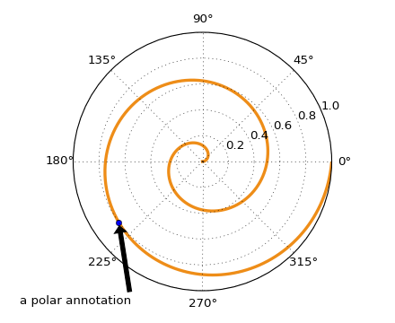
if 1:
# you can specify the xypoint and the xytext in different
# positions and coordinate systems, and optionally turn on a
# connecting line and mark the point with a marker. Annotations
# work on polar axes too. In the example below, the xy point is
# in native coordinates (xycoords defaults to 'data'). For a
# polar axes, this is in (theta, radius) space. The text in this
# example is placed in the fractional figure coordinate system.
# Text keyword args like horizontal and vertical alignment are
# respected
fig = figure()
ax = fig.add_subplot(111, polar=True)
r = np.arange(0,1,0.001)
theta = 2*2*np.pi*r
line, = ax.plot(theta, r, color='#ee8d18', lw=3)
ind = 800
thisr, thistheta = r[ind], theta[ind]
ax.plot([thistheta], [thisr], 'o')
ax.annotate('a polar annotation',
xy=(thistheta, thisr), # theta, radius
xytext=(0.05, 0.05), # fraction, fraction
textcoords='figure fraction',
arrowprops=dict(facecolor='black', shrink=0.05),
horizontalalignment='left',
verticalalignment='bottom',
)
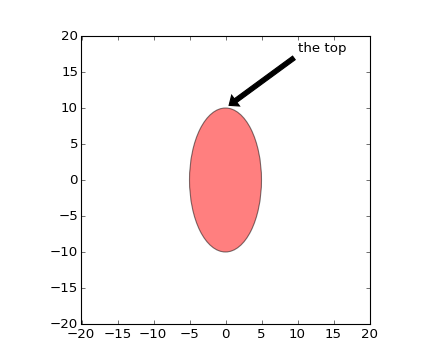
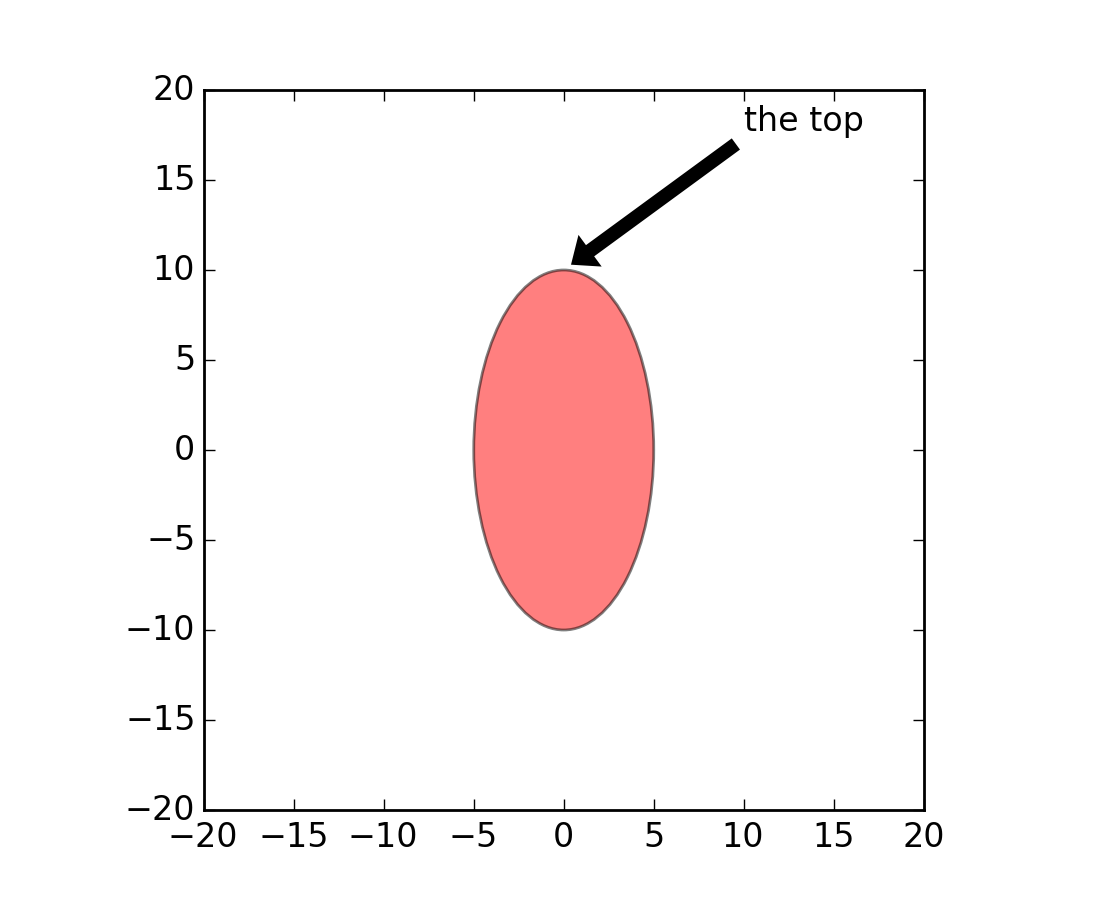
if 1:
# You can also use polar notation on a cartesian axes. Here the
# native coordinate system ('data') is cartesian, so you need to
# specify the xycoords and textcoords as 'polar' if you want to
# use (theta, radius)
el = Ellipse((0,0), 10, 20, facecolor='r', alpha=0.5)
fig = figure()
ax = fig.add_subplot(111, aspect='equal')
ax.add_artist(el)
el.set_clip_box(ax.bbox)
ax.annotate('the top',
xy=(np.pi/2., 10.), # theta, radius
xytext=(np.pi/3, 20.), # theta, radius
xycoords='polar',
textcoords='polar',
arrowprops=dict(facecolor='black', shrink=0.05),
horizontalalignment='left',
verticalalignment='bottom',
clip_on=True, # clip to the axes bounding box
)
ax.set_xlim(-20, 20)
ax.set_ylim(-20, 20)
show()
Keywords: python, matplotlib, pylab, example, codex (see Search examples)
