
"""
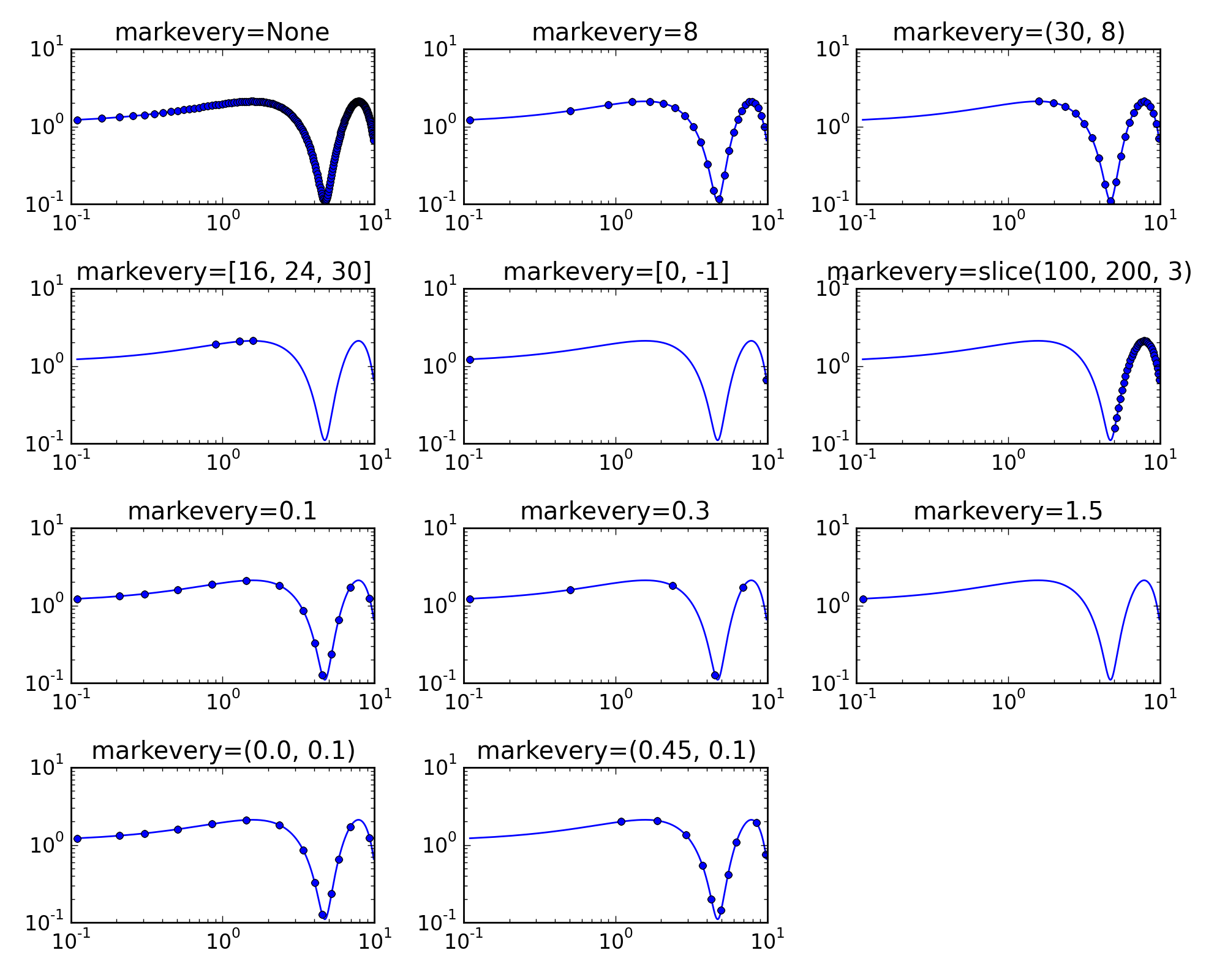
This example demonstrates the various options for showing a marker at a
subset of data points using the `markevery` property of a Line2D object.
Integer arguments are fairly intuitive. e.g. `markevery`=5 will plot every
5th marker starting from the first data point.
Float arguments allow markers to be spaced at approximately equal distances
along the line. The theoretical distance along the line between markers is
determined by multiplying the display-coordinate distance of the axes
bounding-box diagonal by the value of `markevery`. The data points closest
to the theoretical distances will be shown.
A slice or list/array can also be used with `markevery` to specify the markers
to show.
"""
from __future__ import division
import numpy as np
import matplotlib.pyplot as plt
import matplotlib.gridspec as gridspec
#define a list of markevery cases to plot
cases = [None,
8,
(30, 8),
[16, 24, 30], [0,-1],
slice(100,200,3),
0.1, 0.3, 1.5,
(0.0, 0.1), (0.45, 0.1)]
#define the figure size and grid layout properties
figsize = (10, 8)
cols = 3
gs = gridspec.GridSpec(len(cases) // cols + 1, cols)
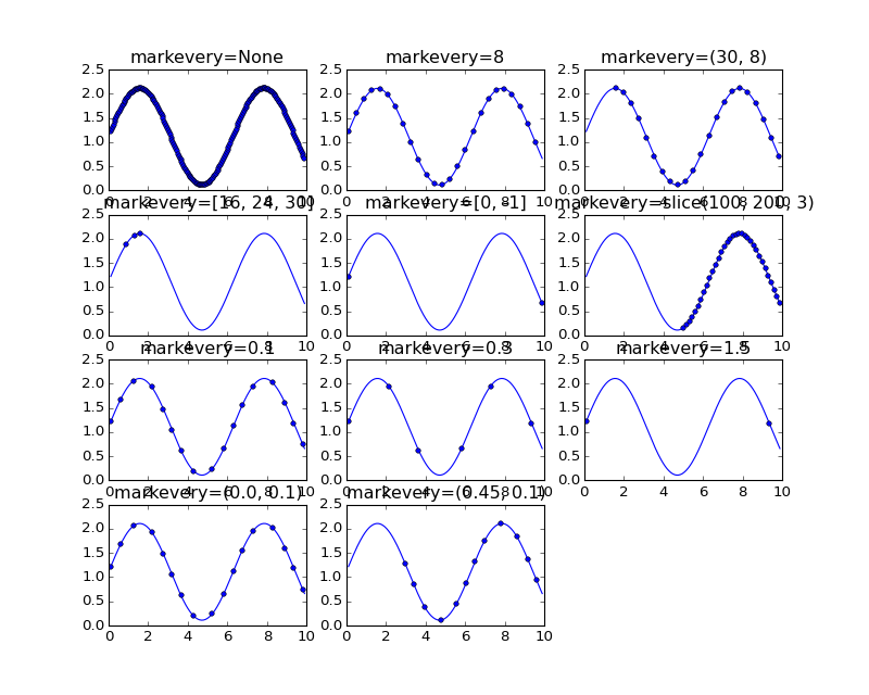
#define the data for cartesian plots
delta = 0.11
x = np.linspace(0, 10 - 2 * delta, 200) + delta
y = np.sin(x) + 1.0 + delta
#plot each markevery case for linear x and y scales
fig1 = plt.figure(num=1, figsize=figsize)
ax = []
for i, case in enumerate(cases):
row = (i // cols)
col = i % cols
ax.append(fig1.add_subplot(gs[row, col]))
ax[-1].set_title('markevery=%s' % str(case))
ax[-1].plot(x, y, 'o', ls='-', ms=4, markevery=case)
#fig1.tight_layout()
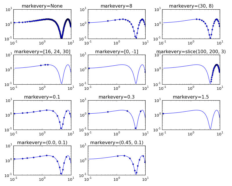
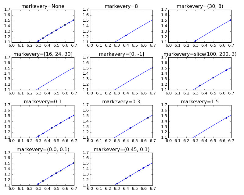
#plot each markevery case for log x and y scales
fig2 = plt.figure(num=2, figsize=figsize)
axlog = []
for i, case in enumerate(cases):
row = (i // cols)
col = i % cols
axlog.append(fig2.add_subplot(gs[row, col]))
axlog[-1].set_title('markevery=%s' % str(case))
axlog[-1].set_xscale('log')
axlog[-1].set_yscale('log')
axlog[-1].plot(x, y, 'o', ls='-', ms=4, markevery=case)
fig2.tight_layout()
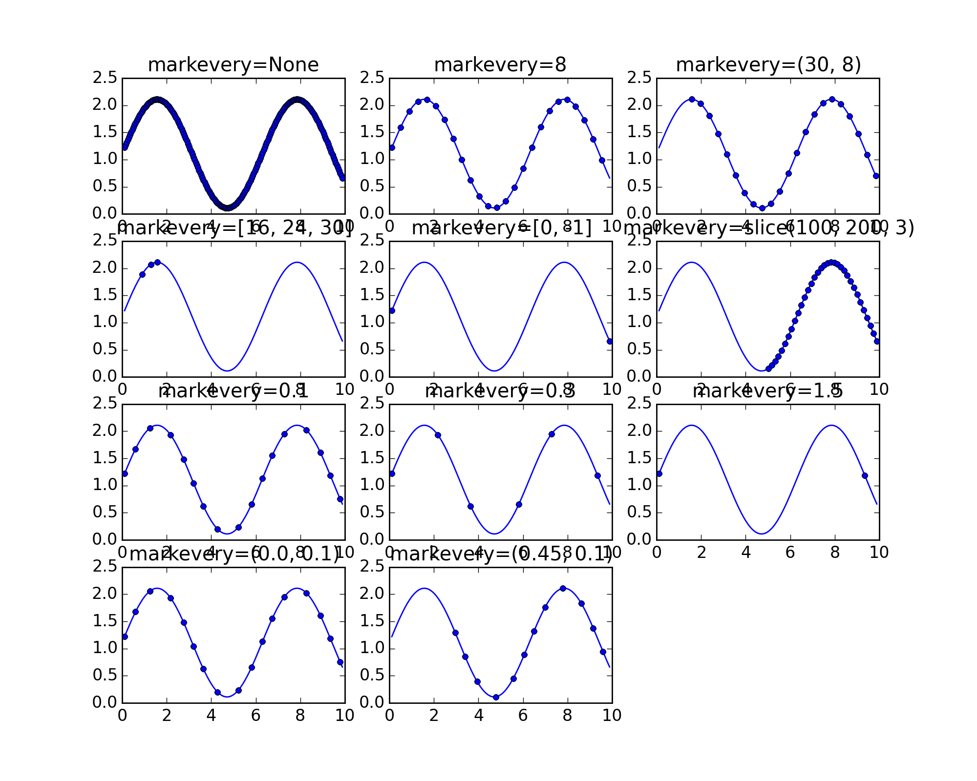
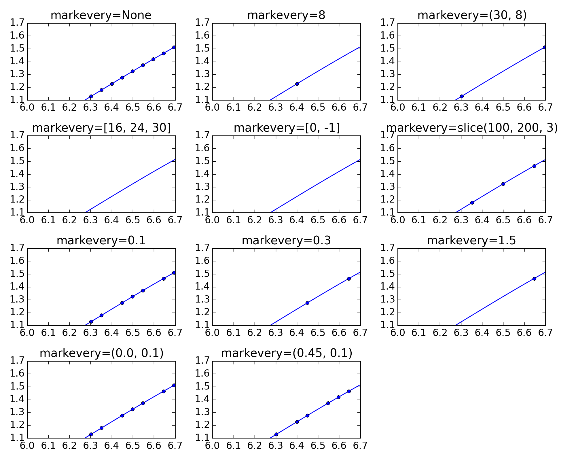
#plot each markevery case for linear x and y scales but zoomed in
#note the behaviour when zoomed in. When a start marker offset is specified
#it is always interpreted with respect to the first data point which might be
#different to the first visible data point.
fig3 = plt.figure(num=3, figsize=figsize)
axzoom = []
for i, case in enumerate(cases):
row = (i // cols)
col = i % cols
axzoom.append(fig3.add_subplot(gs[row, col]))
axzoom[-1].set_title('markevery=%s' % str(case))
axzoom[-1].plot(x, y, 'o', ls='-', ms=4, markevery=case)
axzoom[-1].set_xlim((6, 6.7))
axzoom[-1].set_ylim((1.1, 1.7))
fig3.tight_layout()
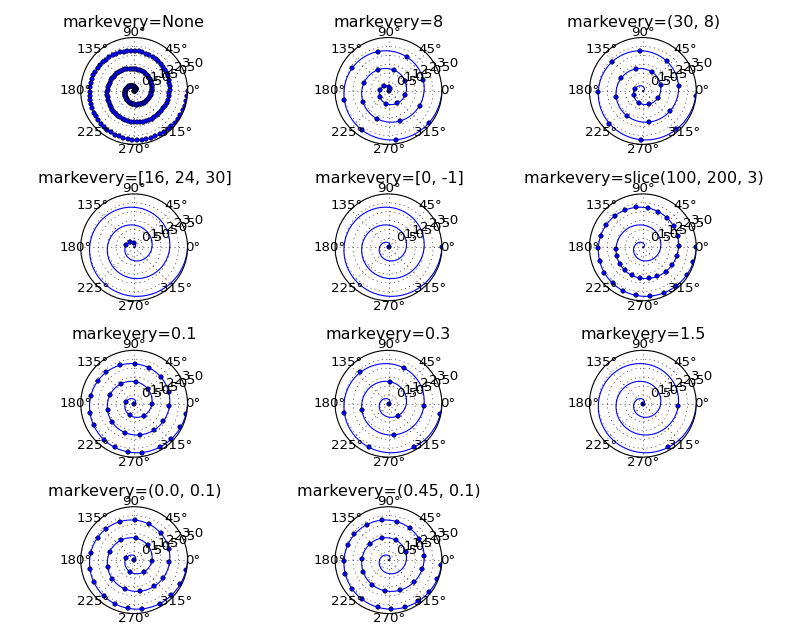
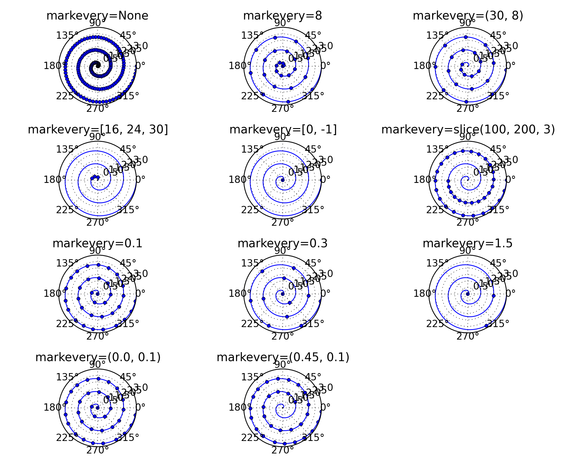
#define data for polar plots
r = np.linspace(0, 3.0, 200)
theta = 2 * np.pi * r
#plot each markevery case for polar plots
fig4 = plt.figure(num=4, figsize=figsize)
axpolar = []
for i, case in enumerate(cases):
row = (i // cols)
col = i % cols
axpolar.append(fig4.add_subplot(gs[row, col], polar = True))
axpolar[-1].set_title('markevery=%s' % str(case))
axpolar[-1].plot(theta, r, 'o', ls='-', ms=4, markevery=case)
fig4.tight_layout()
plt.show()
Keywords: python, matplotlib, pylab, example, codex (see Search examples)

