
#!/usr/bin/env python
import numpy as np
import pylab as P
#
# The hist() function now has a lot more options
#
#
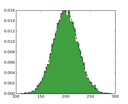
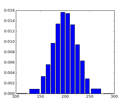
# first create a single histogram
#
mu, sigma = 200, 25
x = mu + sigma*P.randn(10000)
# the histogram of the data with histtype='step'
n, bins, patches = P.hist(x, 50, normed=1, histtype='stepfilled')
P.setp(patches, 'facecolor', 'g', 'alpha', 0.75)
# add a line showing the expected distribution
y = P.normpdf( bins, mu, sigma)
l = P.plot(bins, y, 'k--', linewidth=1.5)
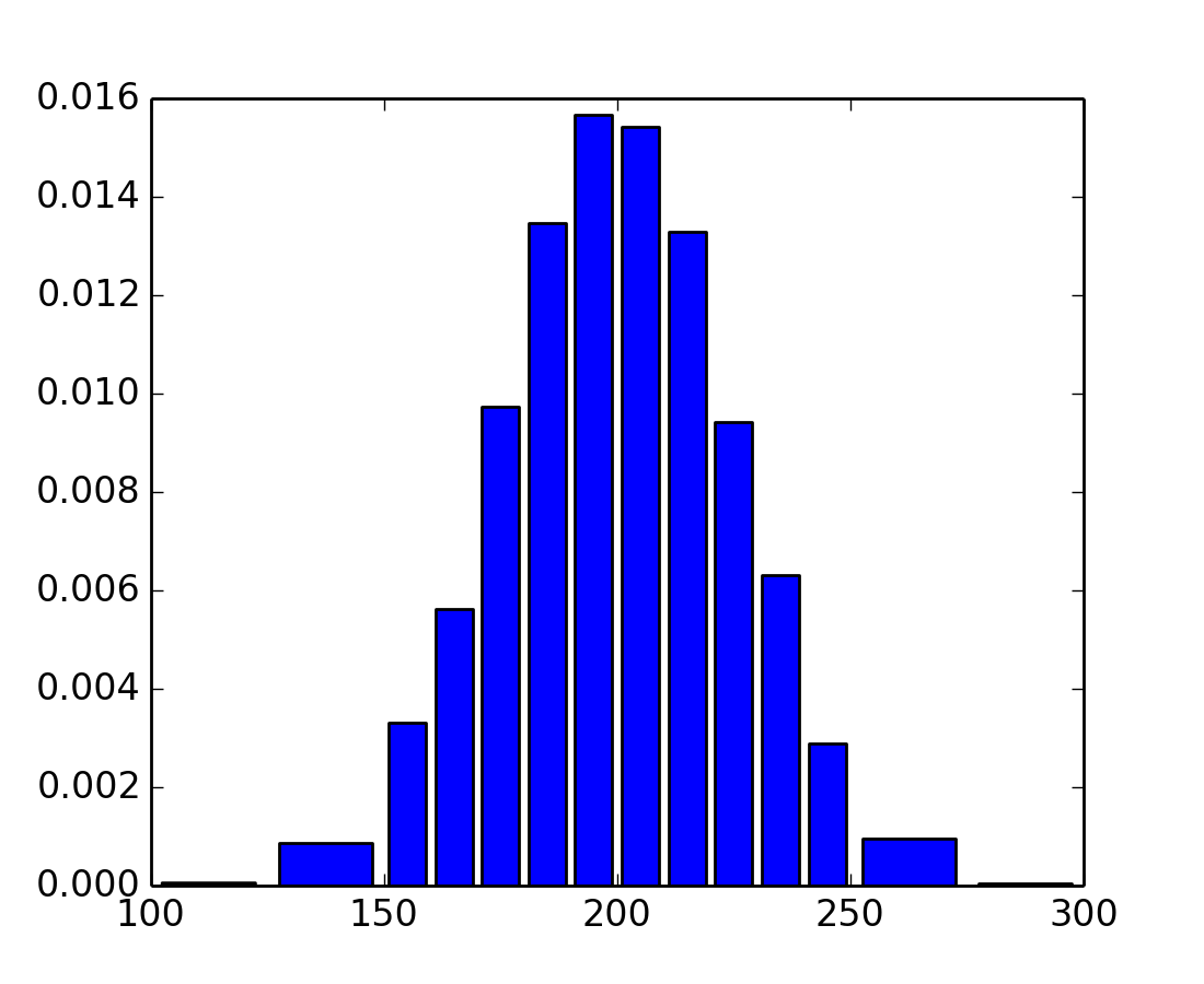
#
# create a histogram by providing the bin edges (unequally spaced)
#
P.figure()
bins = [100,125,150,160,170,180,190,200,210,220,230,240,250,275,300]
# the histogram of the data with histtype='step'
n, bins, patches = P.hist(x, bins, normed=1, histtype='bar', rwidth=0.8)
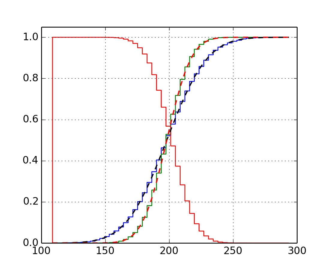
#
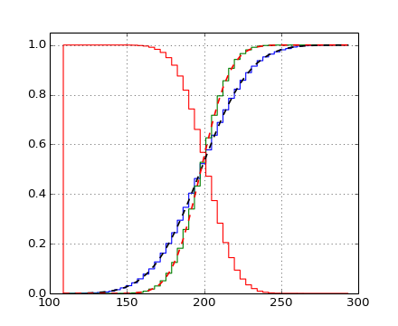
# now we create a cumulative histogram of the data
#
P.figure()
n, bins, patches = P.hist(x, 50, normed=1, histtype='step', cumulative=True)
# add a line showing the expected distribution
y = P.normpdf( bins, mu, sigma).cumsum()
y /= y[-1]
l = P.plot(bins, y, 'k--', linewidth=1.5)
# create a second data-set with a smaller standard deviation
sigma2 = 15.
x = mu + sigma2*P.randn(10000)
n, bins, patches = P.hist(x, bins=bins, normed=1, histtype='step', cumulative=True)
# add a line showing the expected distribution
y = P.normpdf( bins, mu, sigma2).cumsum()
y /= y[-1]
l = P.plot(bins, y, 'r--', linewidth=1.5)
# finally overplot a reverted cumulative histogram
n, bins, patches = P.hist(x, bins=bins, normed=1,
histtype='step', cumulative=-1)
P.grid(True)
P.ylim(0, 1.05)
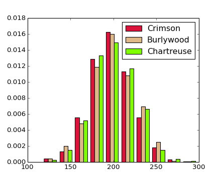
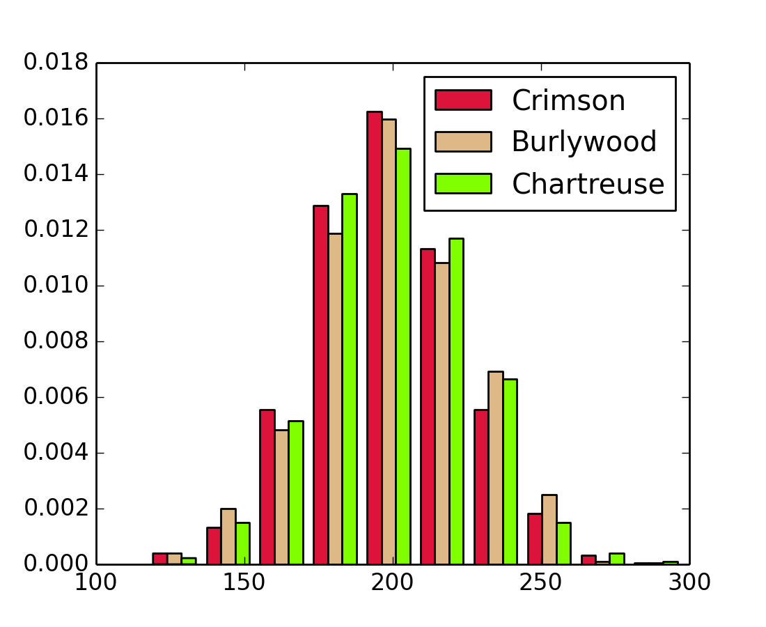
#
# histogram has the ability to plot multiple data in parallel ...
# Note the new color kwarg, used to override the default, which
# uses the line color cycle.
#
P.figure()
# create a new data-set
x = mu + sigma*P.randn(1000,3)
n, bins, patches = P.hist(x, 10, normed=1, histtype='bar',
color=['crimson', 'burlywood', 'chartreuse'],
label=['Crimson', 'Burlywood', 'Chartreuse'])
P.legend()
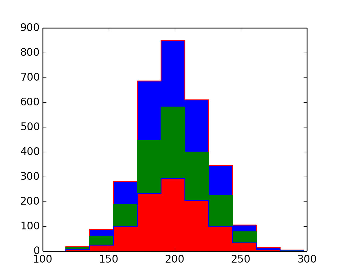
#
# ... or we can stack the data
#
P.figure()
n, bins, patches = P.hist(x, 10, normed=1, histtype='bar', stacked=True)
P.show()
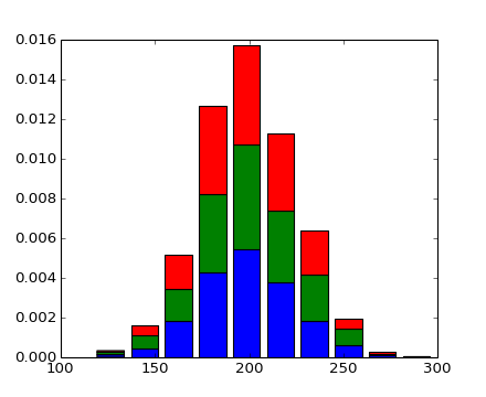
#
# we can also stack using the step histtype
#
P.figure()
n, bins, patches = P.hist(x, 10, histtype='step', stacked=True, fill=True)
P.show()
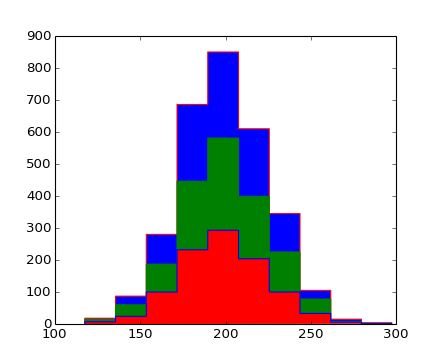
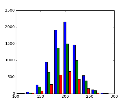
#
# finally: make a multiple-histogram of data-sets with different length
#
x0 = mu + sigma*P.randn(10000)
x1 = mu + sigma*P.randn(7000)
x2 = mu + sigma*P.randn(3000)
# and exercise the weights option by arbitrarily giving the first half
# of each series only half the weight of the others:
w0 = np.ones_like(x0)
w0[:len(x0)/2] = 0.5
w1 = np.ones_like(x1)
w1[:len(x1)/2] = 0.5
w2 = np.ones_like(x2)
w2[:len(x2)/2] = 0.5
P.figure()
n, bins, patches = P.hist( [x0,x1,x2], 10, weights=[w0, w1, w2], histtype='bar')
P.show()
Keywords: python, matplotlib, pylab, example, codex (see Search examples)


