viz API Reference¶

probscale.viz.probplot(data, ax=None, plottype='prob', dist=None, probax='x', problabel=None, datascale='linear', datalabel=None, bestfit=False, return_best_fit_results=False, estimate_ci=False, ci_kws=None, pp_kws=None, scatter_kws=None, line_kws=None, **fgkwargs)[source]¶

Probability, percentile, and quantile plots.

Parameters:	data : array-like 1-dimensional data to be plotted ax : matplotlib axes, optional The Axes on which to plot. If one is not provided, a new Axes will be created. plottype : string (default = ‘prob’) Type of plot to be created. Options are: ‘prob’: probabilty plot ‘pp’: percentile plot ‘qq’: quantile plot dist : scipy distribution, optional A distribtion to compute the scale’s tick positions. If not specified, a standard normal distribution will be used. probax : string, optional (default = ‘x’) The axis (‘x’ or ‘y’) that will serve as the probability (or quantile) axis. problabel, datalabel : string, optional Axis labels for the probability/quantile and data axes respectively. datascale : string, optional (default = ‘log’) Scale for the other axis that is not bestfit : bool, optional (default is False) Specifies whether a best-fit line should be added to the plot. return_best_fit_results : bool (default is False) If True a dictionary of results of is returned along with the figure. estimate_ci : bool, optional (False) Estimate and draw a confidence band around the best-fit line using a percentile bootstrap. ci_kws : dict, optional Dictionary of keyword arguments passed directly to viz.fit_line when computing the best-fit line. pp_kws : dict, optional Dictionary of keyword arguments passed directly to viz.plot_pos when computing the plotting positions. scatter_kws, line_kws : dict, optional Dictionary of keyword arguments passed directly to ax.plot when drawing the scatter points and best-fit line, respectively.
Returns:	fig : matplotlib.Figure The figure on which the plot was drawn. result : dict of linear fit results, optional Keys are: q : array of quantiles x, y : arrays of data passed to function xhat, yhat : arrays of modeled data plotted in best-fit line res : array of coeffcients of the best-fit line.
Other Parameters:
	color : string, optional A directly-specified matplotlib color argument for both the data series and the best-fit line if drawn. This argument is made available for compatibility for the seaborn package and is not recommended for general use. Instead colors should be specified within scatter_kws and line_kws. Note Users should not specify this parameter. It is inteded to only be used by seaborn when operating within a FacetGrid. label : string, optional A directly-specified legend label for the data series. This argument is made available for compatibility for the seaborn package and is not recommended for general use. Instead the data series label should be specified within scatter_kws. Note Users should not specify this parameter. It is inteded to only be used by seaborn when operating within a FacetGrid.

See also

viz.plot_pos, viz.fit_line, numpy.polyfit, scipy.stats.probplot, scipy.stats.mstats.plotting_positions

Examples

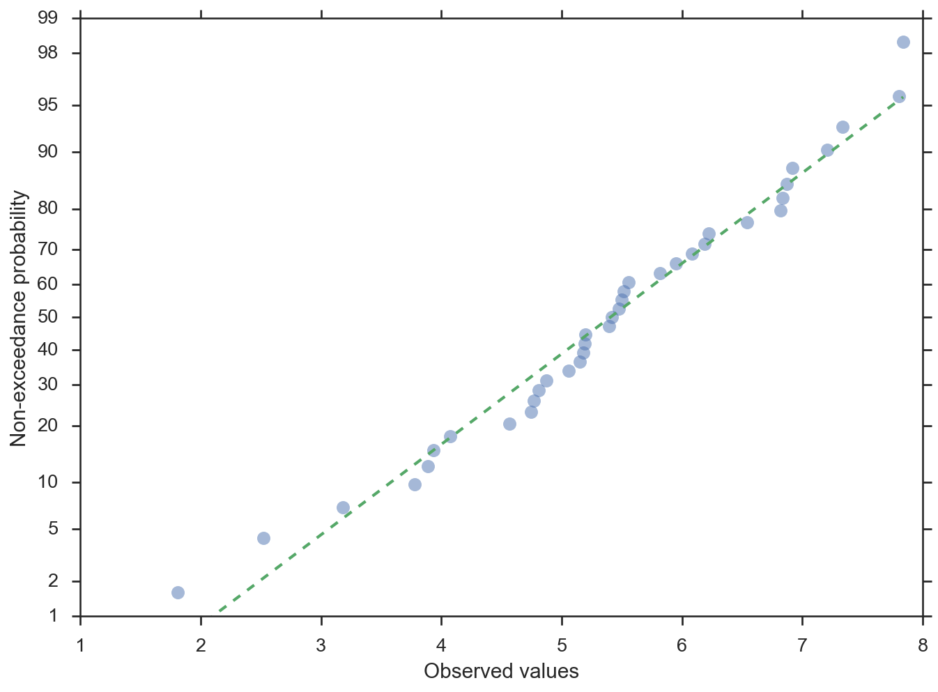
Probability plot with the probabilities on the y-axis

>>> import numpy; numpy.random.seed(0)
>>> from matplotlib import pyplot
>>> from scipy import stats
>>> from probscale.viz import probplot
>>> data = numpy.random.normal(loc=5, scale=1.25, size=37)
>>> fig = probplot(data, plottype='prob', probax='y',
...          problabel='Non-exceedance probability',
...          datalabel='Observed values', bestfit=True,
...          line_kws=dict(linestyle='--', linewidth=2),
...          scatter_kws=dict(marker='o', alpha=0.5))

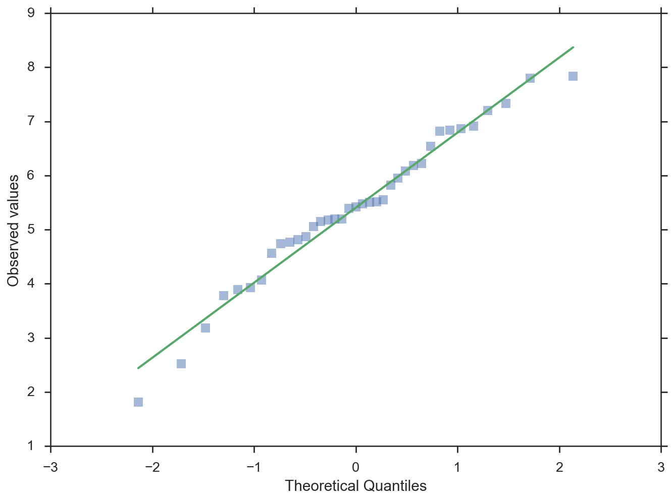
Quantile plot with the quantiles on the x-axis

>>> fig = probplot(data, plottype='qq', probax='x',
...          problabel='Theoretical Quantiles',
...          datalabel='Observed values', bestfit=True,
...          line_kws=dict(linestyle='-', linewidth=2),
...          scatter_kws=dict(marker='s', alpha=0.5))

probscale.viz.plot_pos(data, postype=None, alpha=None, beta=None)[source]¶

Compute the plotting positions for a dataset. Heavily borrows from scipy.stats.mstats.plotting_positions.

A plottiting position is defined as: (i-alpha)/(n+1-alpha-beta) where:

• i is the rank order
• n is the size of the dataset
• alpha and beta are parameters used to adjust the positions.

The values of alpha and beta can be explicitly set. Typical values can also be access via the postype parameter. Available postype values (alpha, beta) are:

“type 4” (alpha=0, beta=1)

Linear interpolation of the empirical CDF.

“type 5” or “hazen” (alpha=0.5, beta=0.5)

Piecewise linear interpolation.

“type 6” or “weibull” (alpha=0, beta=0)

Weibull plotting positions. Unbiased exceedance probability for all distributions. Recommended for hydrologic applications.

“type 7” (alpha=1, beta=1)

The default values in R. Not recommended with probability scales as the min and max data points get plotting positions of 0 and 1, respectively, and therefore cannot be shown.

“type 8” (alpha=1/3, beta=1/3)

Approximately median-unbiased.

“type 9” or “blom” (alpha=0.375, beta=0.375)

Approximately unbiased positions if the data are normally distributed.

“median” (alpha=0.3175, beta=0.3175)

Median exceedance probabilities for all distributions (used in scipy.stats.probplot).

“apl” or “pwm” (alpha=0.35, beta=0.35)

Used with probability-weighted moments.

“cunnane” (alpha=0.4, beta=0.4)

Nearly unbiased quantiles for normally distributed data. This is the default value.

“gringorten” (alpha=0.44, beta=0.44)

Used for Gumble distributions.

Parameters:	data : array-like The values whose plotting positions need to be computed. postype : string, optional (default: “cunnane”) alpha, beta : float, optional Custom plotting position parameters is the options available through the postype parameter are insufficient.
Returns:	plot_pos : numpy.array The computed plotting positions, sorted. data_sorted : numpy.array The original data values, sorted.

References

http://artax.karlin.mff.cuni.cz/r-help/library/lmomco/html/pp.html http://astrostatistics.psu.edu/su07/R/html/stats/html/quantile.html http://docs.scipy.org/doc/scipy-0.17.0/reference/generated/scipy.stats.probplot.html http://docs.scipy.org/doc/scipy-0.17.0/reference/generated/scipy.stats.mstats.plotting_positions.html

probscale.viz.fit_line(x, y, xhat=None, fitprobs=None, fitlogs=None, dist=None, estimate_ci=False, niter=10000, alpha=0.05)[source]¶

Fits a line to x-y data in various forms (linear, log, prob scales).

Parameters:

x, y : array-like Independent and dependent data, respectively. xhat : array-like, optional The values at which yhat should should be estimated. If not provided, falls back to the sorted values of x. fitprobs, fitlogs : str, optional. Defines how data should be transformed. Valid values are ‘x’, ‘y’, or ‘both’. If using fitprobs, variables should be expressed as a percentage, i.e., for a probablility transform, data will be transformed with lambda x: dist.ppf(x / 100.). For a log transform, lambda x: numpy.log(x). Take care to not pass the same value to both fitlogs and figprobs as both transforms will be applied. dist : distribution, optional A fully-spec’d scipy.stats distribution-like object such that dist.ppf and dist.cdf can be called. If not provided, defaults to a minimal implementation of scipt.stats.norm. estimate_ci : bool, optional (False) Estimate and draw a confidence band around the best-fit line using a percentile bootstrap. niter : int, optional (default = 10000) Number of bootstrap iterations if estimate_ci is provided. alpha : float, optional (default = 0.05) The confidence level of the bootstrap estimate.

Returns:

xhat, yhat : numpy arrays Linear model estimates of x and y. results : dict Dictionary of linear fit results. Keys include: slope intersept yhat_lo (lower confidence interval of the estimated y-vals) yhat_hi (upper confidence interval of the estimated y-vals)